File to load Ler dispersal data
Here is the new file data/disperseLer.R:
### Creates the data object disperseLer, representing the Ler dispersal experiment

# Get data from Jenn's file
data_dir <- "~/Dropbox/Arabidopsis/analysis"
disperseLer <- read.csv(file.path(data_dir, '2013_08_08_Exp1_Spray.csv'),
                        header = TRUE)

# Drop the "clipped" treatment
disperseLer <- droplevels(subset(disperseLer, new_trt != "clipped", drop = TRUE))

# Drop the columns with the (irrelevant) info about where the mom pots came from
disperseLer <- disperseLer[, -c(1:4, 6)]

# Clean up column names
names(disperseLer) <- c("ID", "Pot", "Distance", "Seedlings", "Siliques", "Density",
                        "Treatment")

# Make some factor variables
disperseLer$ID <- as.factor(disperseLer$ID)

# Clean up the workspace
rm(data_dir)

# Auto-cache the data
ProjectTemplate::cache("disperseLer")
Summarizing Ler dispersal data
Here is a file to summarize the data by replicate, in lib/helpers.R:
calc_dispersal_stats <- function(dispersal_data) {
  dispersal_stats <- group_by(dispersal_data, ID, Density, Siliques) %>%
    summarise(
      Total_seeds = sum(Seedlings),
      Home_seeds = Seedlings[1],
      Dispersing_seeds = Total_seeds - Home_seeds,
      Dispersal_fraction = Dispersing_seeds / Total_seeds,
      # Dispersal stats including all seeds
      Mean_dispersal_all = sum(Seedlings * (Distance - 4)) / Total_seeds,
      RMS_dispersal_all = sqrt(sum(Seedlings * (Distance - 4)^2) / Total_seeds),
      # Dispersal stats including just dispersing seeds
      Mean_dispersal = sum(Seedlings * (Distance - 4)) / Dispersing_seeds,
      RMS_dispersal = sqrt(sum(Seedlings * (Distance - 4)^2) / Dispersing_seeds)
    )
  return (dispersal_stats)
}
Let’s look at how the total seed number, the fraction dispersing, and the dispersal distances scale with density:
Ler_dispersal_stats <- calc_dispersal_stats(disperseLer)
qplot(Density, Total_seeds, data = Ler_dispersal_stats)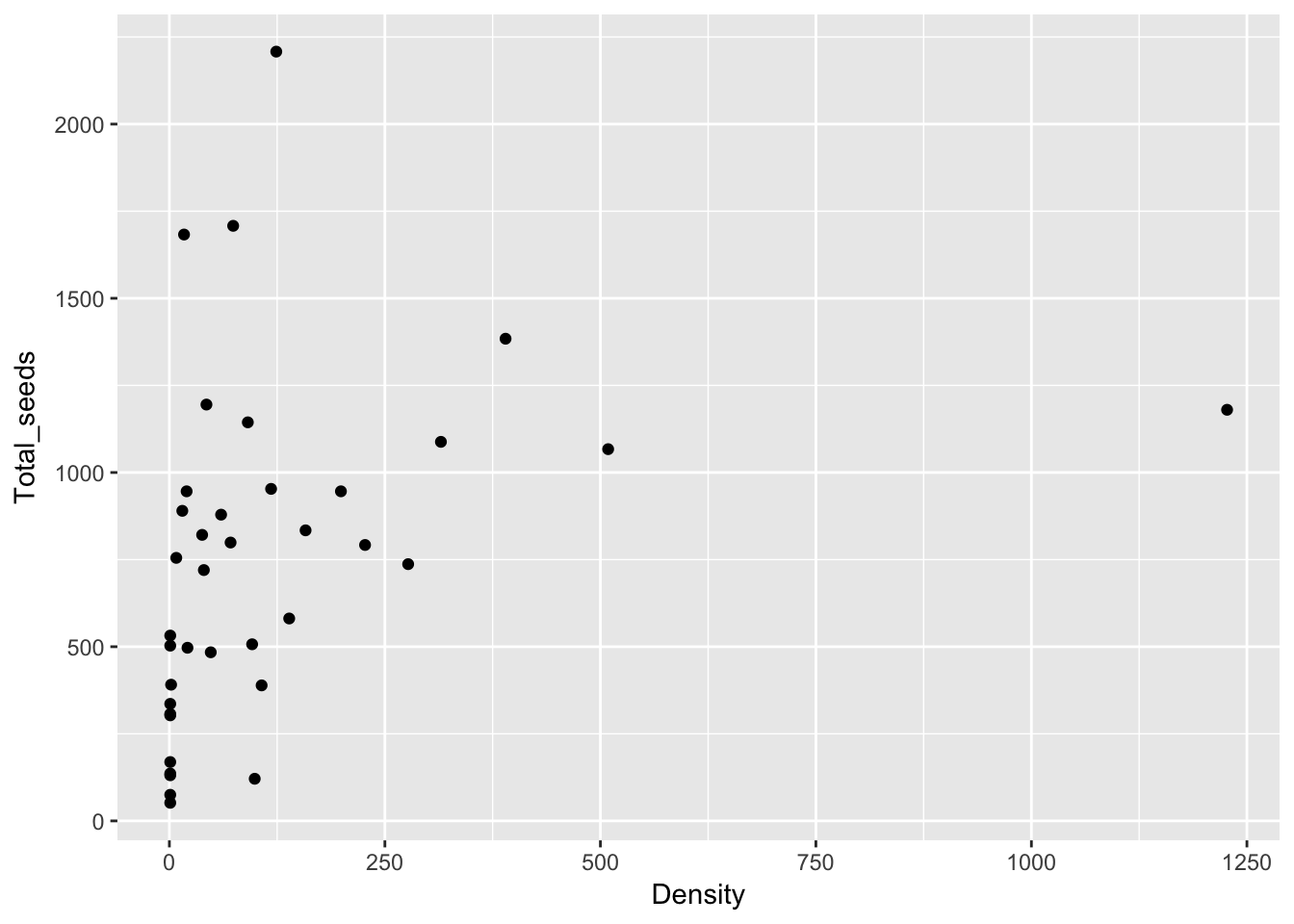
qplot(Density, Dispersal_fraction, data = Ler_dispersal_stats)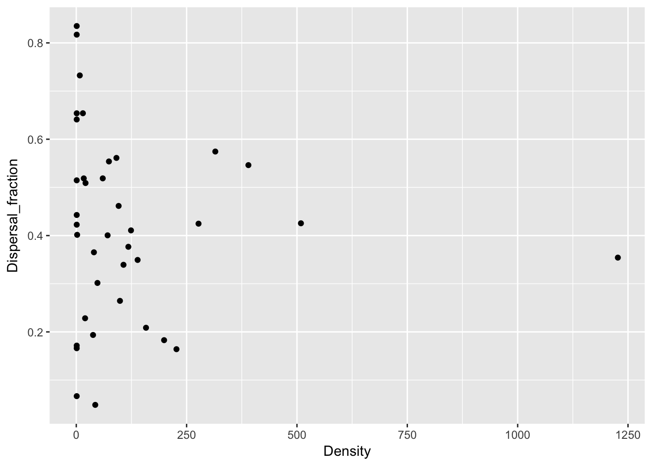
qplot(Density, Mean_dispersal_all, data = Ler_dispersal_stats)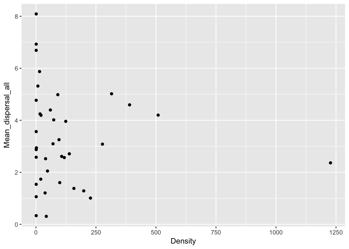
qplot(Density, Mean_dispersal, data = Ler_dispersal_stats)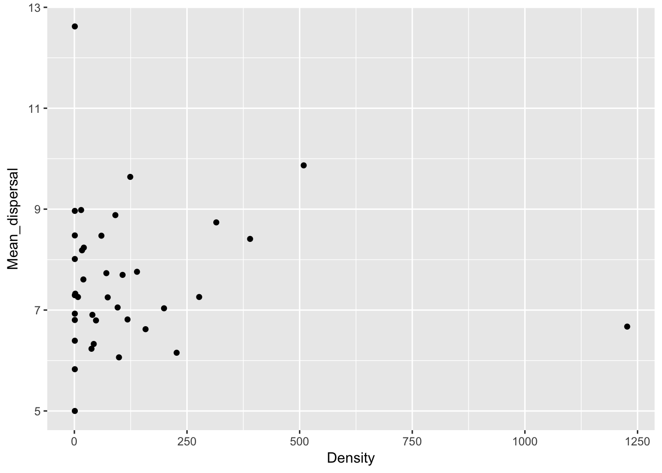
qplot(Density, RMS_dispersal_all, data = Ler_dispersal_stats)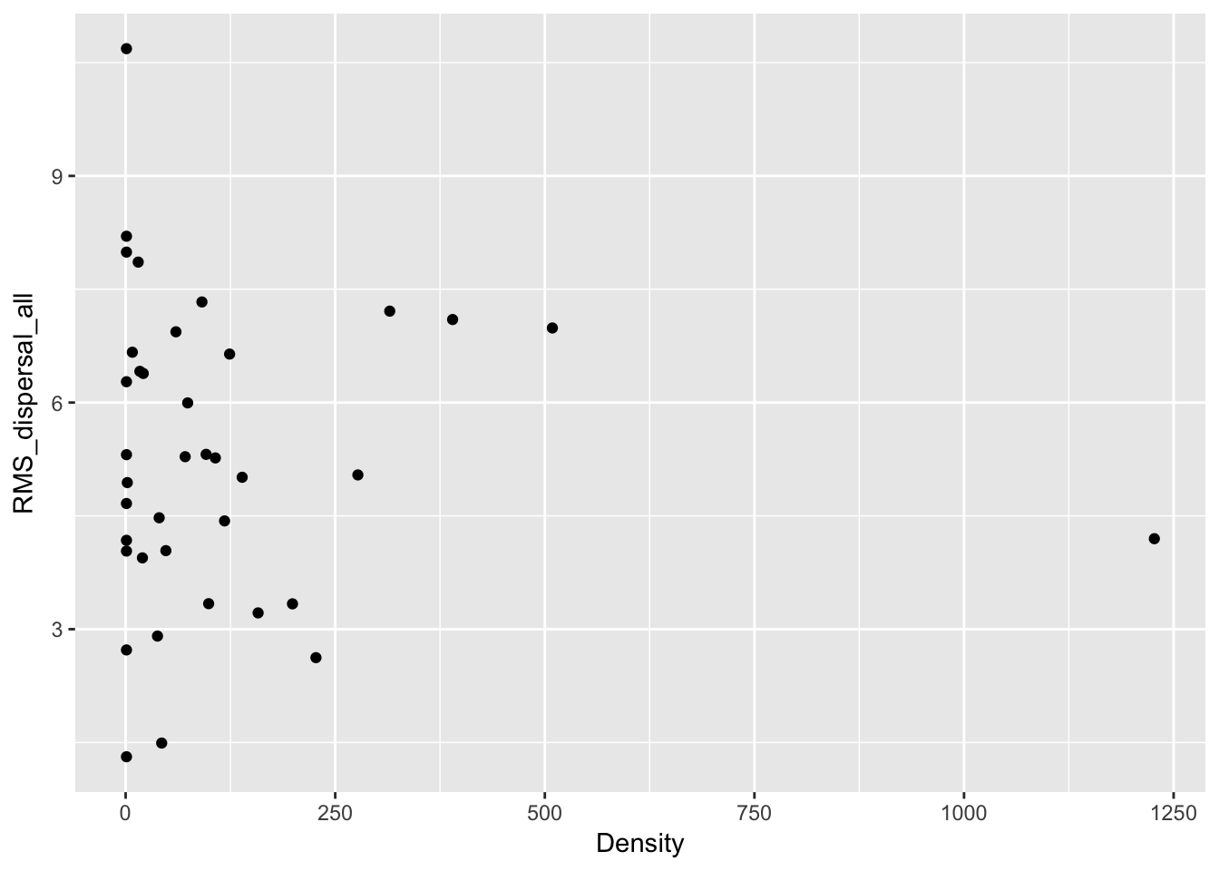
qplot(Density, RMS_dispersal, data = Ler_dispersal_stats)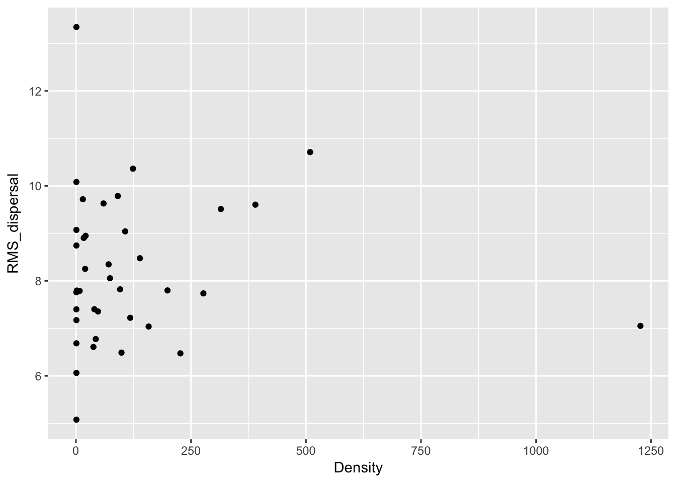
Except for total seed number, there don’t seem to be any patterns here. For the single plants, let’s look at whether silique number (which might be correlated with plant size) can predict anything:
qplot(Siliques, Total_seeds, data = subset(Ler_dispersal_stats, !is.na(Siliques)))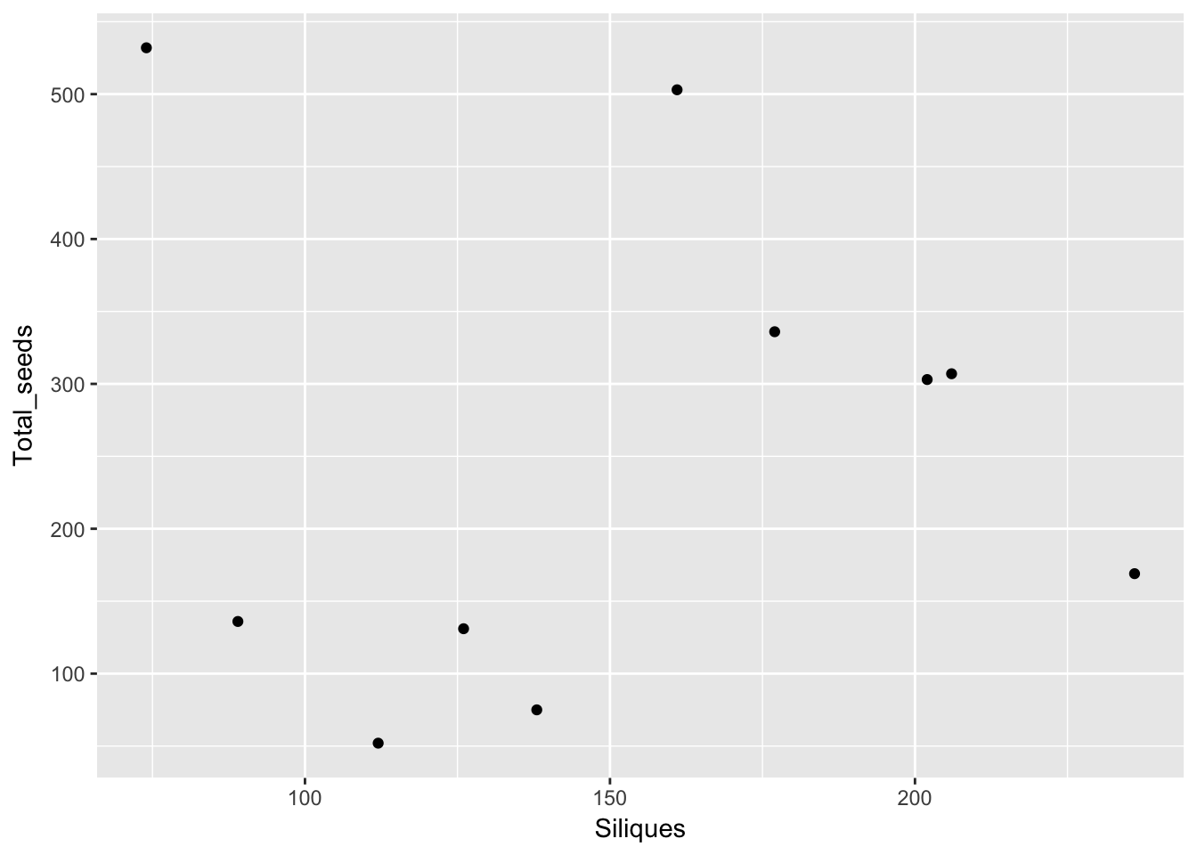
qplot(Siliques, Dispersal_fraction, data = subset(Ler_dispersal_stats, !is.na(Siliques)))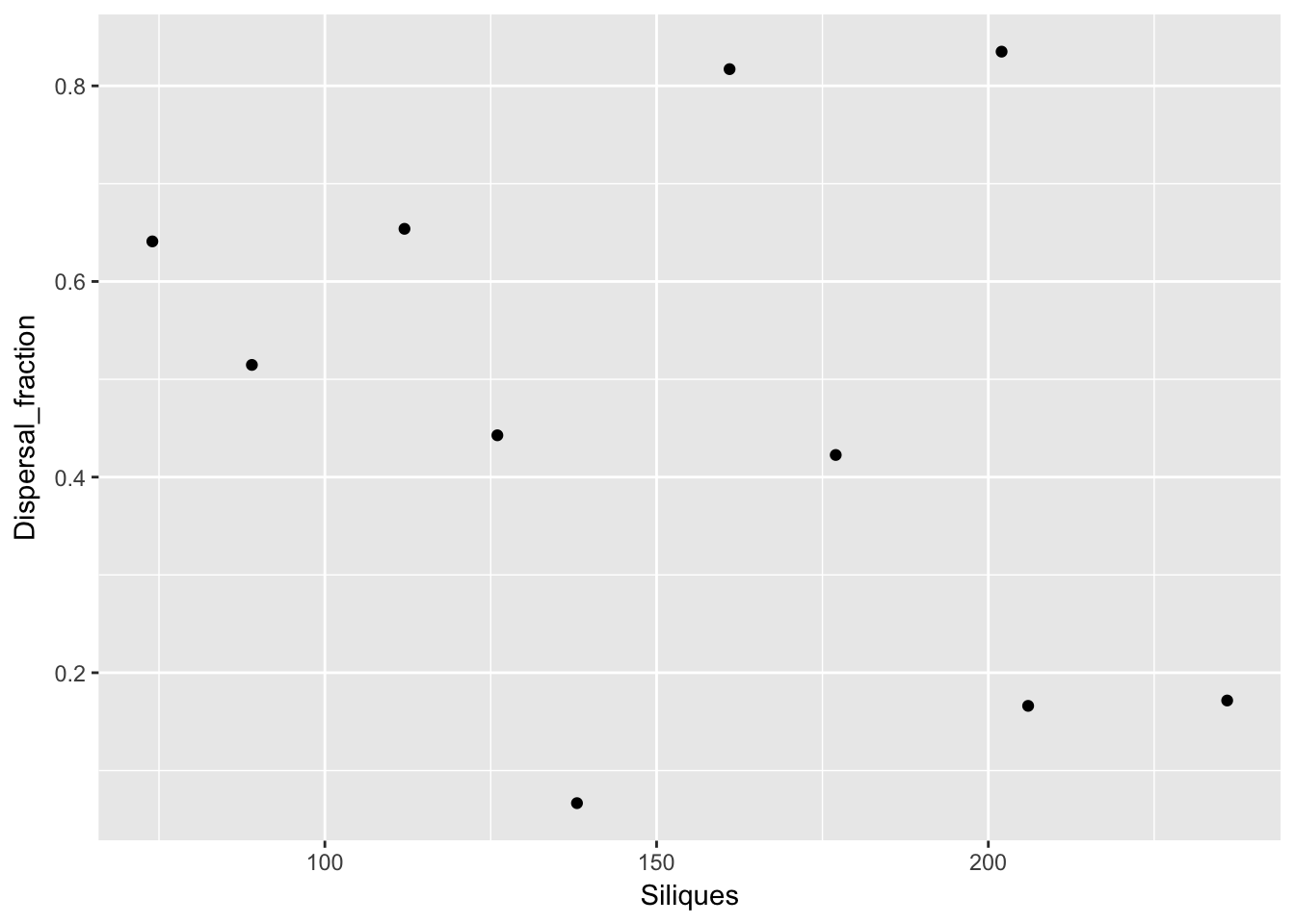
qplot(Siliques, Mean_dispersal_all, data = subset(Ler_dispersal_stats, !is.na(Siliques)))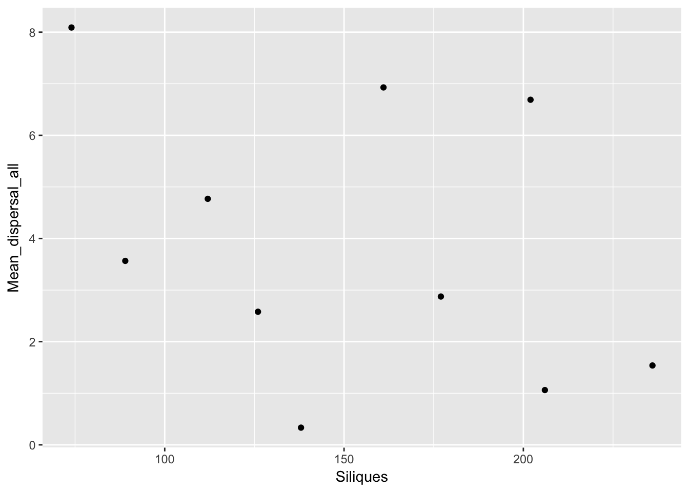
qplot(Siliques, Mean_dispersal, data = subset(Ler_dispersal_stats, !is.na(Siliques)))
qplot(Siliques, RMS_dispersal_all, data = subset(Ler_dispersal_stats, !is.na(Siliques)))
qplot(Siliques, RMS_dispersal, data = subset(Ler_dispersal_stats, !is.na(Siliques)))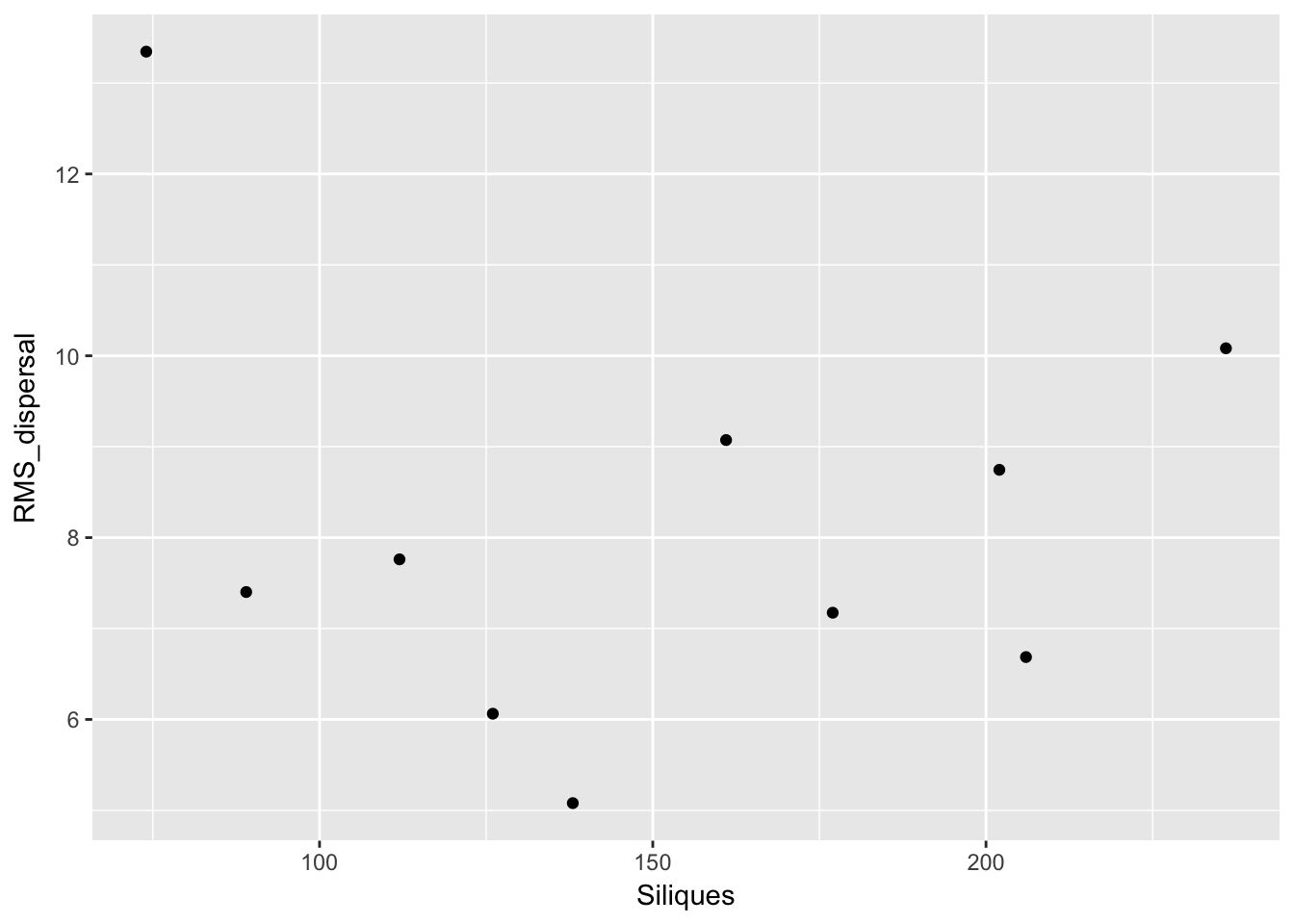
Again, no patterns. This makes modeling simpler!
One more thing to look at: are the mean dispersal distances correlated with either the fraction dispersing or the number of dispersing seeds?
qplot(Dispersing_seeds, Mean_dispersal, data = Ler_dispersal_stats)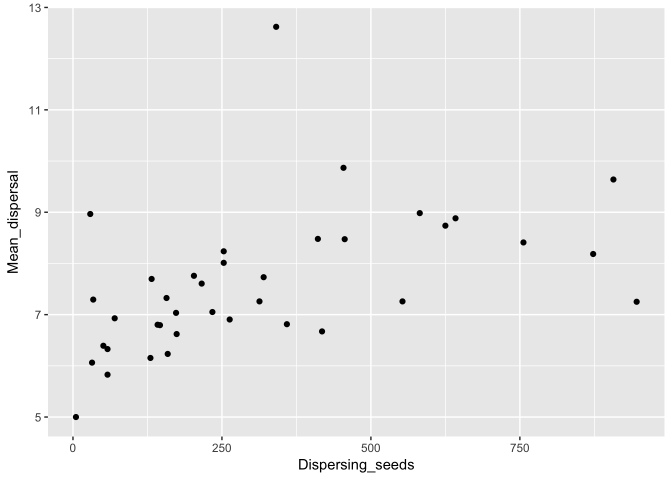
qplot(Dispersing_seeds, RMS_dispersal, data = Ler_dispersal_stats)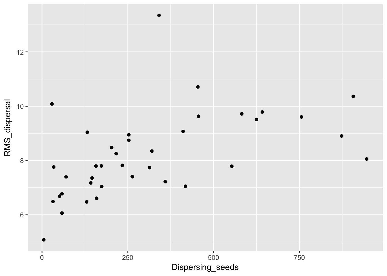
qplot(Dispersal_fraction, Mean_dispersal, data = Ler_dispersal_stats)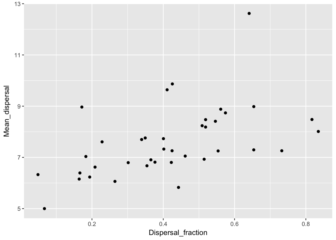
qplot(Dispersal_fraction, RMS_dispersal, data = Ler_dispersal_stats)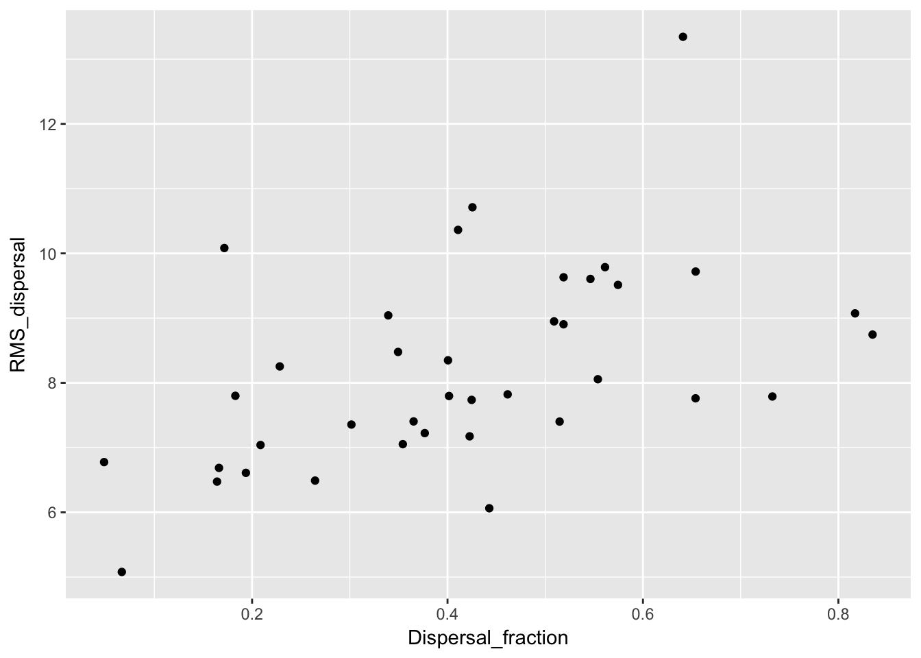 Here we see a correlation with both. This could just be a sampling effect; once we fit kernel parameters we’ll have to see if they have correlations as well. If so, that suggests that the same variables (such as canopy height and structure, and intensity of simulated rainfall) that affect whether seeds leave the home pot also affect how far they go.
Here’s a multiple regression just to tease out the two variables:
summary(lm(Mean_dispersal ~ Dispersal_fraction + Dispersing_seeds, data = Ler_dispersal_stats))
Call:
lm(formula = Mean_dispersal ~ Dispersal_fraction + Dispersing_seeds,
    data = Ler_dispersal_stats)

Residuals:
    Min      1Q  Median      3Q     Max
-1.7144 -0.5299 -0.2285  0.3843  4.4228

Coefficients:
                    Estimate Std. Error t value Pr(>|t|)
(Intercept)        6.0255317  0.4449107  13.543 1.76e-15 ***
Dispersal_fraction 2.5229534  1.1204944   2.252   0.0307 *
Dispersing_seeds   0.0016311  0.0008397   1.942   0.0602 .
---
Signif. codes:  0 '***' 0.001 '**' 0.01 '*' 0.05 '.' 0.1 ' ' 1

Residual standard error: 1.148 on 35 degrees of freedom
Multiple R-squared:  0.3358,    Adjusted R-squared:  0.2979
F-statistic: 8.849 on 2 and 35 DF,  p-value: 0.000776
summary(lm(RMS_dispersal ~ Dispersal_fraction + Dispersing_seeds, data = Ler_dispersal_stats))
Call:
lm(formula = RMS_dispersal ~ Dispersal_fraction + Dispersing_seeds,
    data = Ler_dispersal_stats)

Residuals:
    Min      1Q  Median      3Q     Max
-1.8021 -0.6943 -0.3313  0.5148  4.4709

Coefficients:
                    Estimate Std. Error t value Pr(>|t|)
(Intercept)        6.4639884  0.5020757  12.875 7.77e-15 ***
Dispersal_fraction 2.6898597  1.2644627   2.127   0.0405 *
Dispersing_seeds   0.0020128  0.0009476   2.124   0.0408 *
---
Signif. codes:  0 '***' 0.001 '**' 0.01 '*' 0.05 '.' 0.1 ' ' 1

Residual standard error: 1.296 on 35 degrees of freedom
Multiple R-squared:  0.3415,    Adjusted R-squared:  0.3039
F-statistic: 9.076 on 2 and 35 DF,  p-value: 0.0006679
It appears that both are playing a role. But the dispersal fraction is a stronger predictor, which suggests that there is real mechanism here, and not just sampling getting further into the kernel.
Kernel fitting issues
Our data are actually interval-censored, and we need to ensure that we are taking that into account. I believe that the likelihood functions I wrote previously take that into account, but they lack the rigor of fitdistrplus. Unfortunately, the data have another issue: the seeds in pot zero are a mixture of “non-dispersers” (i.e., seeds that fall straight down and aren’t part of the kernel) and “short-distance dispersers” (seeds moving according to a dispersal kernel, but traveling less than 3 cm). To account for this either requires writing a zero-inflated distribution (which will require custom functions for everything) or telling the objective function to truncate the distribution. Again I believe that my prior functions do the latter, but I’m not truly confident of that. Unfortunately, there doesn’t seem to be an obvious way to account this in fitdistrplus using out-of-the-box distributions.
Actually, I take that back—the issue of truncation is addressed in the FAQs. It does require writing new distribution functions, but they are pretty straightforward. Here is their example for a (doubly) truncated exponential distribution:
dtexp <- function(x, rate, low, upp)
{
  PU <- pexp(upp, rate=rate)
  PL <- pexp(low, rate=rate)
  dexp(x, rate) / (PU-PL) * (x >= low) * (x <= upp)
}
ptexp <- function(q, rate, low, upp)
{
  PU <- pexp(upp, rate=rate)
  PL <- pexp(low, rate=rate)
  (pexp(q, rate)-PL) / (PU-PL) * (q >= low) * (q <= upp) + 1 * (q > upp)
}
Looking at the dispersal patterns
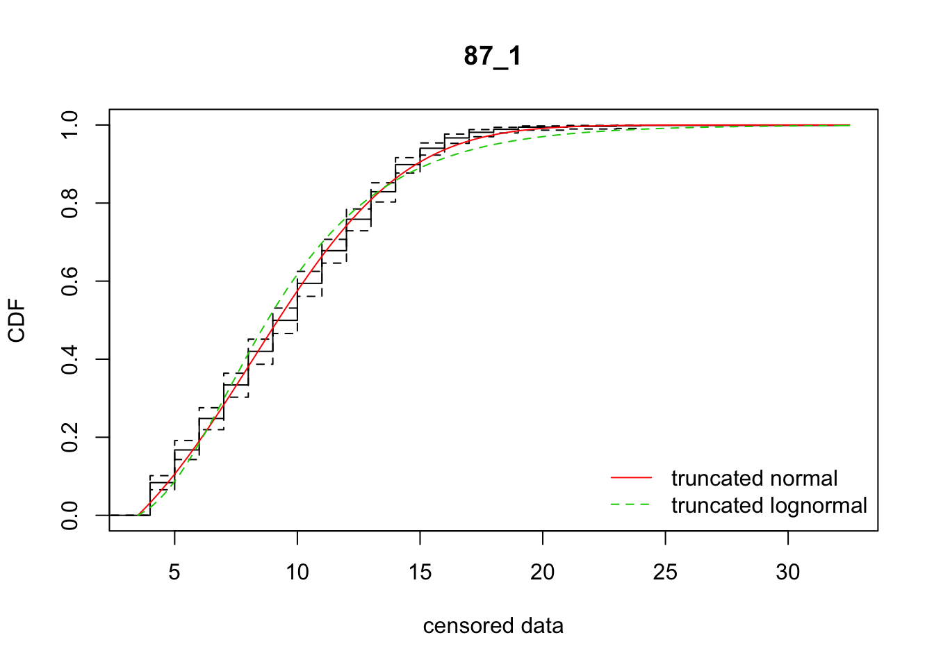
Let’s start by just plotting the raw data. The first plot is just the empirical kernels; the second puts the vertical axis on a log scale (so exponential distributions should look linear and normal distributions should look quadratic) and the third puts both axes on a log scale (so lognormal distributions should look quadratic).
ggplot(aes(x = Distance, y = Seedlings), data = subset(disperseLer, Distance > 4)) +
geom_line() + facet_wrap(~ID, scales = "free_y") 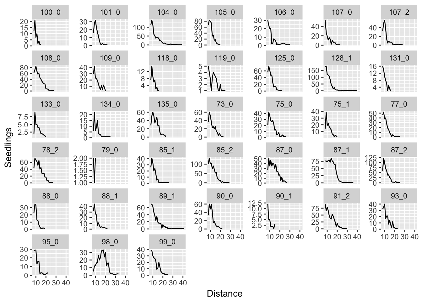
ggplot(aes(x = Distance, y = Seedlings), data = subset(disperseLer, Distance > 4)) +
  geom_line() + facet_wrap(~ID, scales = "free_y") + scale_y_log10()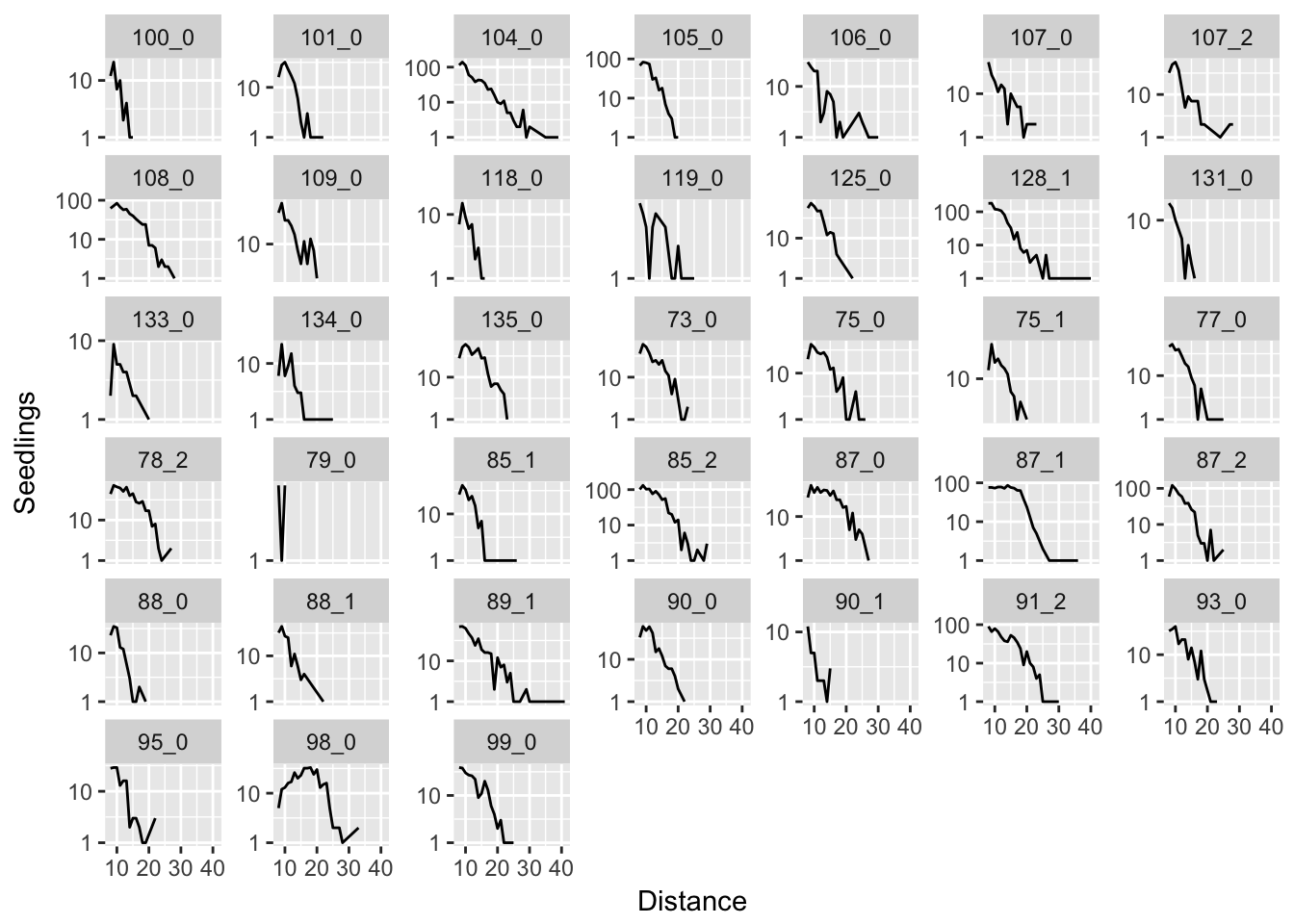
ggplot(aes(x = Distance, y = Seedlings), data = subset(disperseLer, Distance > 4)) +
  geom_line() + facet_wrap(~ID, scales = "free_y") + scale_y_log10() + scale_x_log10()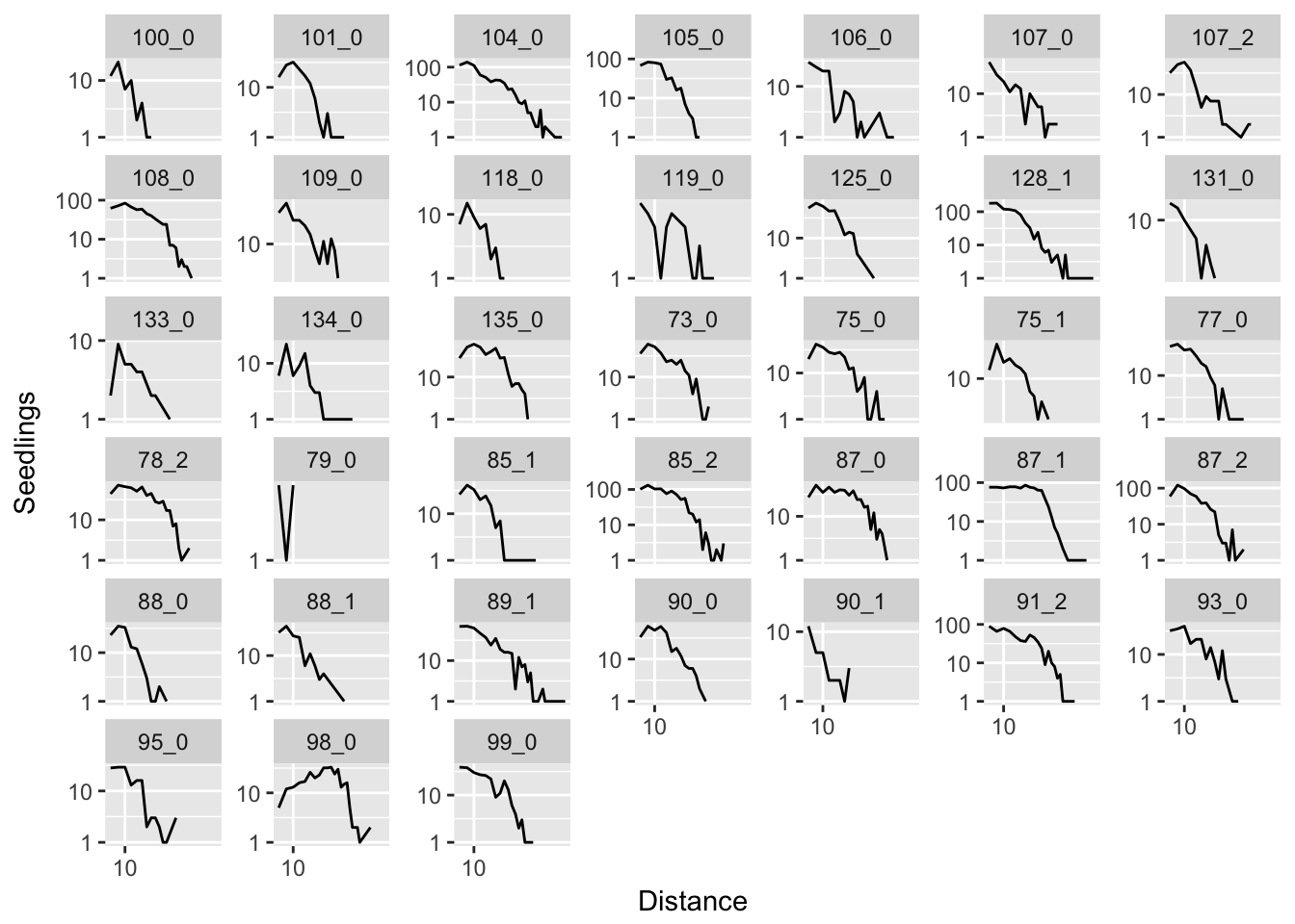
In many cases, it seems like a (truncated) normal distribution might be best! Rep 87_1 is going to be particularly problematic, as it is strongly sigmoid.
Trial fitting
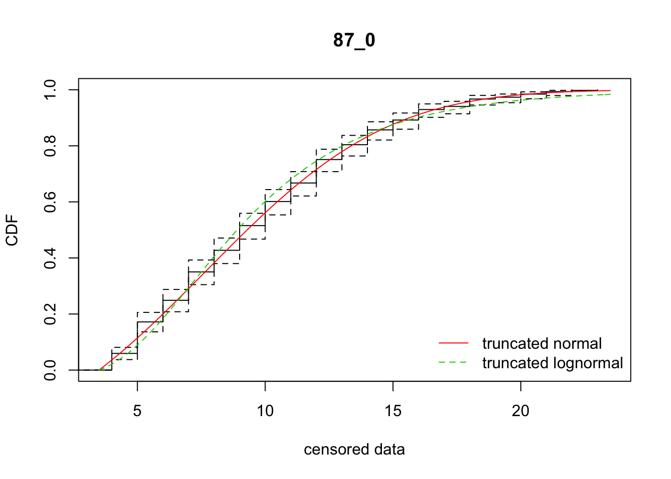
I’ll start by selecting a single rep with a large number of seeds and a well-behaved distribution. Let’s use 87_0.
Pull out the data and convert into the format required by fitdistrplus:
data_87_0 <- subset(disperseLer, ID == "87_0" & Distance > 4)
data_vec <- rep(data_87_0$Distance, data_87_0$Seedlings)
cens_data_tble <- data.frame(left = data_vec - 4.5, right = data_vec - 3.5)
Now construct the distribution functions for a truncated normal. I code in the “standard” truncation level.
dtnorm <- function(x, mean, sd, low = 3.5)
{
  PU <- 1
  PL <- pnorm(low, mean = mean, sd = sd)
  dnorm(x, mean, sd) / (PU-PL) * (x >= low)
}
ptnorm <- function(q, mean, sd, low = 3.5)
{
  PU <- 1
  PL <- pnorm(low, mean = mean, sd = sd)
  (pnorm(q, mean, sd)-PL) / (PU-PL) * (q >= low)
}
So now let’s give it a try:
library(fitdistrplus)
fit_tnorm <- fitdistcens(cens_data_tble, "tnorm", start = list(mean = 6, sd = 10))
summary(fit_tnorm)
Fitting of the distribution ' tnorm ' By maximum likelihood on censored data
Parameters
estimate Std. Error
mean 7.681504 0.5930568
sd 5.588817 0.3661223
Fixed parameters:
data frame with 0 columns and 0 rows
Loglikelihood: -1242.553 AIC: 2489.106 BIC: 2497.343
Correlation matrix:
mean sd
mean 1.000000 -0.803976
sd -0.803976 1.000000cdfcompcens(fit_tnorm, Turnbull.confint = TRUE)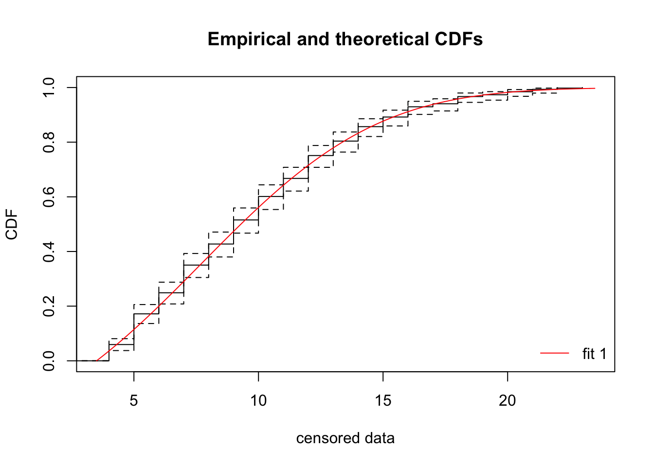 This looks like a pretty darn good fit!
Interestingly, using the non-censored method gives almost identical parameter estimates and CDF:
fit3<-fitdist(data_vec - 4, "tnorm", start = list(mean = 6, sd = 10))
summary(fit3)
Fitting of the distribution ' tnorm ' by maximum likelihood
Parameters :
estimate Std. Error
mean 7.696363 0.5870556
sd 5.583054 0.3626565
Loglikelihood: -1242.376 AIC: 2488.752 BIC: 2496.988
Correlation matrix:
mean sd
mean 1.000000 -0.801385
sd -0.801385 1.000000cdfcomp(fit3)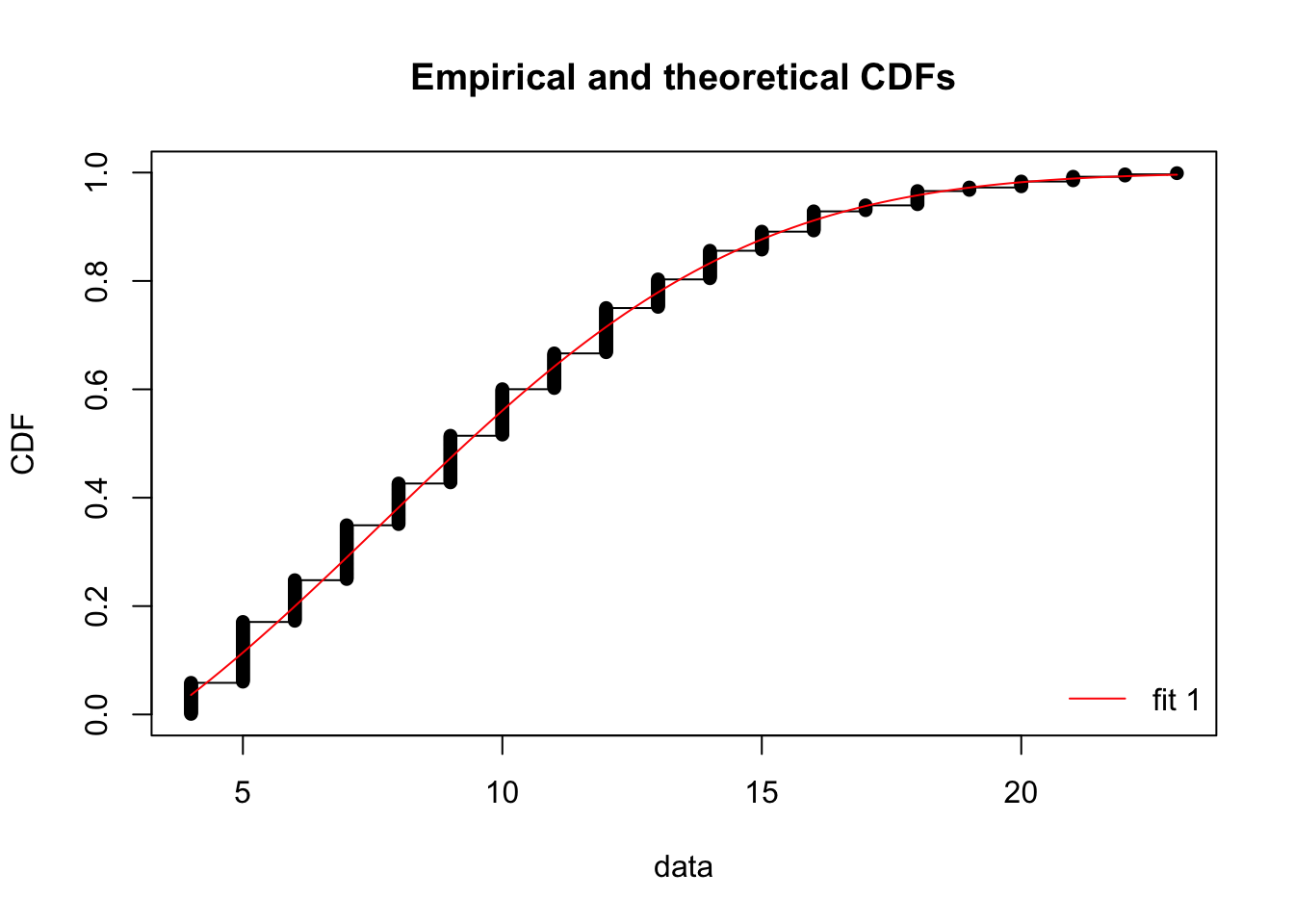
Thus, we can use some of the other diagnostic plots for non-censored data:
denscomp(fit3, breaks = 3:23+0.5, plotstyle = "ggplot", xlim = c(3, 24))
# qqcomp(fit3) # This one requires defining a quantile function!
ppcomp(fit3)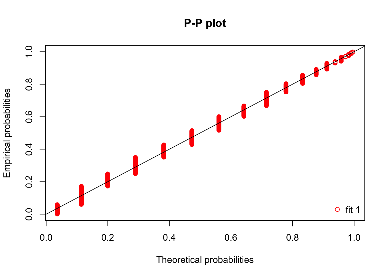 Unfortunately, we need additional work to get qqcomp working; and denscomp only gives a sensible looking histogram with tweaking (and even there, the bins are not centered appropriately, so the histogram is shifted).
Here’s a rough draft of a better figure:
xx = seq(3.3, max(fit3$data) + 0.7, 0.1)
plot(xx, (dtnorm(xx, fit3$estimate[1], fit3$estimate[2])), type = "l", col="red")
points(table(fit3$data)/length(fit3$data))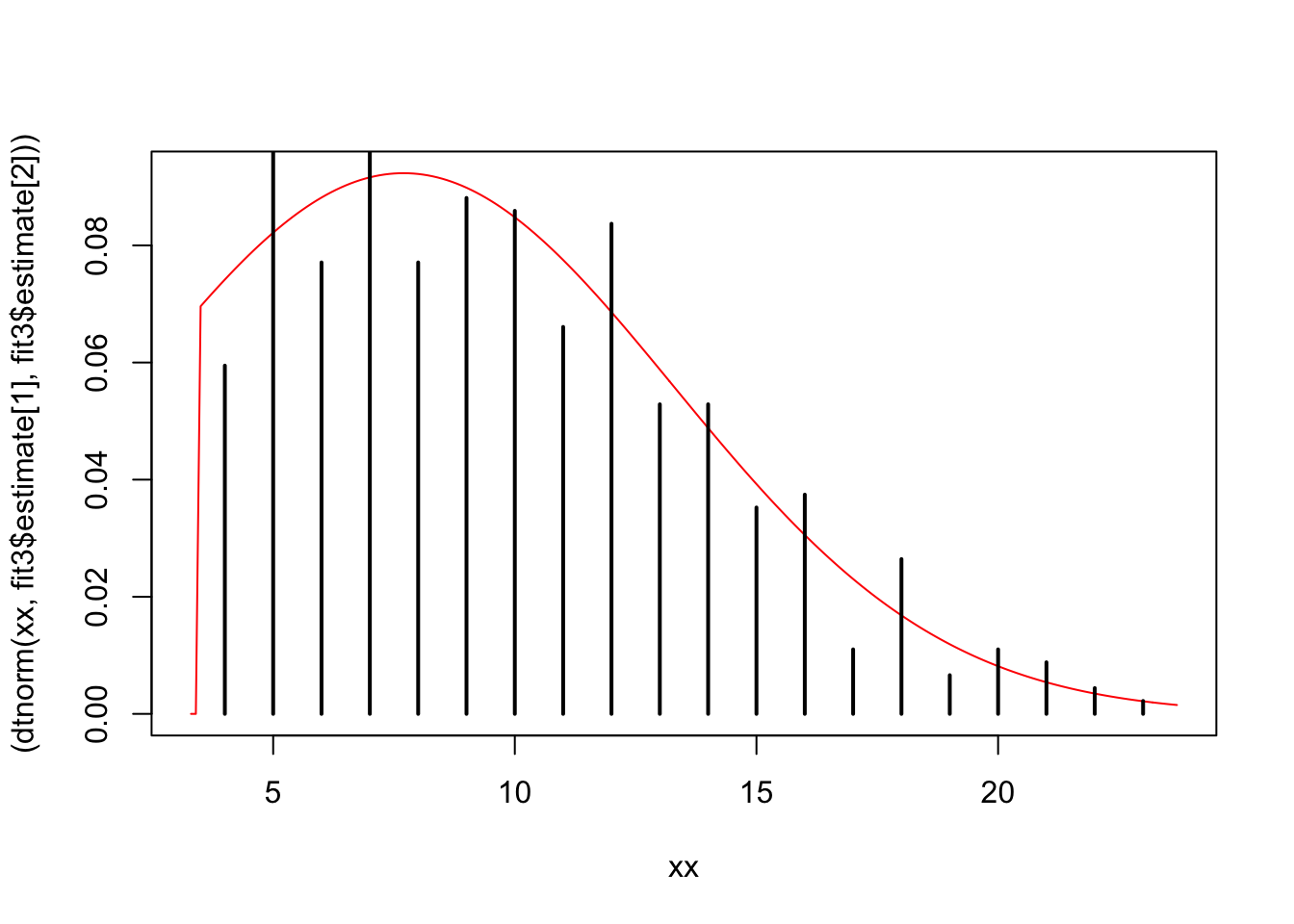
We can make analagous functions for the log normal distribution:
dtlnorm <- function(x, meanlog, sdlog, low = 3.5)
{
  PU <- 1
  PL <- plnorm(low, meanlog = meanlog, sdlog = sdlog)
  dlnorm(x, meanlog, sdlog) / (PU-PL) * (x >= low)
}
ptlnorm <- function(q, meanlog, sdlog, low = 3.5)
{
  PU <- 1
  PL <- plnorm(low, meanlog = meanlog, sdlog = sdlog)
  (plnorm(q, meanlog, sdlog)-PL) / (PU-PL) * (q >= low)
}
Now fit to the censored data and compare with our normal fit
fit_tlnorm <- fitdistcens(cens_data_tble, "tlnorm", start = list(meanlog = log(6), sdlog = log(10)))
summary(fit_tlnorm)
Fitting of the distribution ' tlnorm ' By maximum likelihood on censored data
Parameters
estimate Std. Error
meanlog 2.1737212 0.02373376
sdlog 0.4584419 0.01879380
Fixed parameters:
data frame with 0 columns and 0 rows
Loglikelihood: -1254.488 AIC: 2512.976 BIC: 2521.212
Correlation matrix:
meanlog sdlog
meanlog 1.0000000 -0.2594226
sdlog -0.2594226 1.0000000cdfcompcens(list(fit_tnorm, fit_tlnorm), Turnbull.confint = TRUE,
legendtext = c("truncated normal", "truncated lognormal"))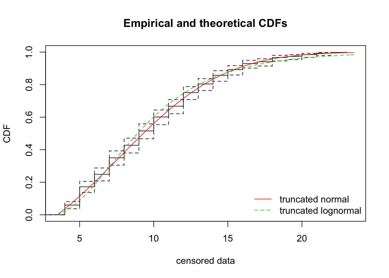
The CDF of the log-normal is not as good, and the AIC is about 24 units worse.
Fit all the replicates
Start by writing a function that takes a single replicate’s data and does the analysis
fit_dispersal_models <- function(dispersal_data) {
data_loc <- subset(dispersal_data, Distance > 4)
data_vec <- rep(data_loc$Distance, data_loc$Seedlings)
cens_data_tble <- data.frame(left = data_vec - 4.5, right = data_vec - 3.5)
fit_tnorm <- fitdistcens(cens_data_tble, "tnorm", start = list(mean = 6, sd = 10))
fit_tlnorm <- fitdistcens(cens_data_tble, "tlnorm", start = list(meanlog = log(6), sdlog = log(10)))
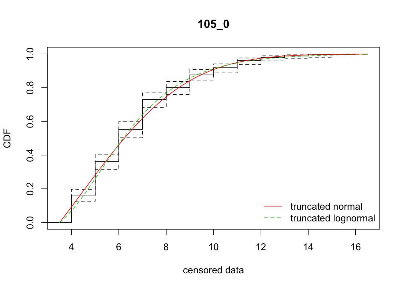
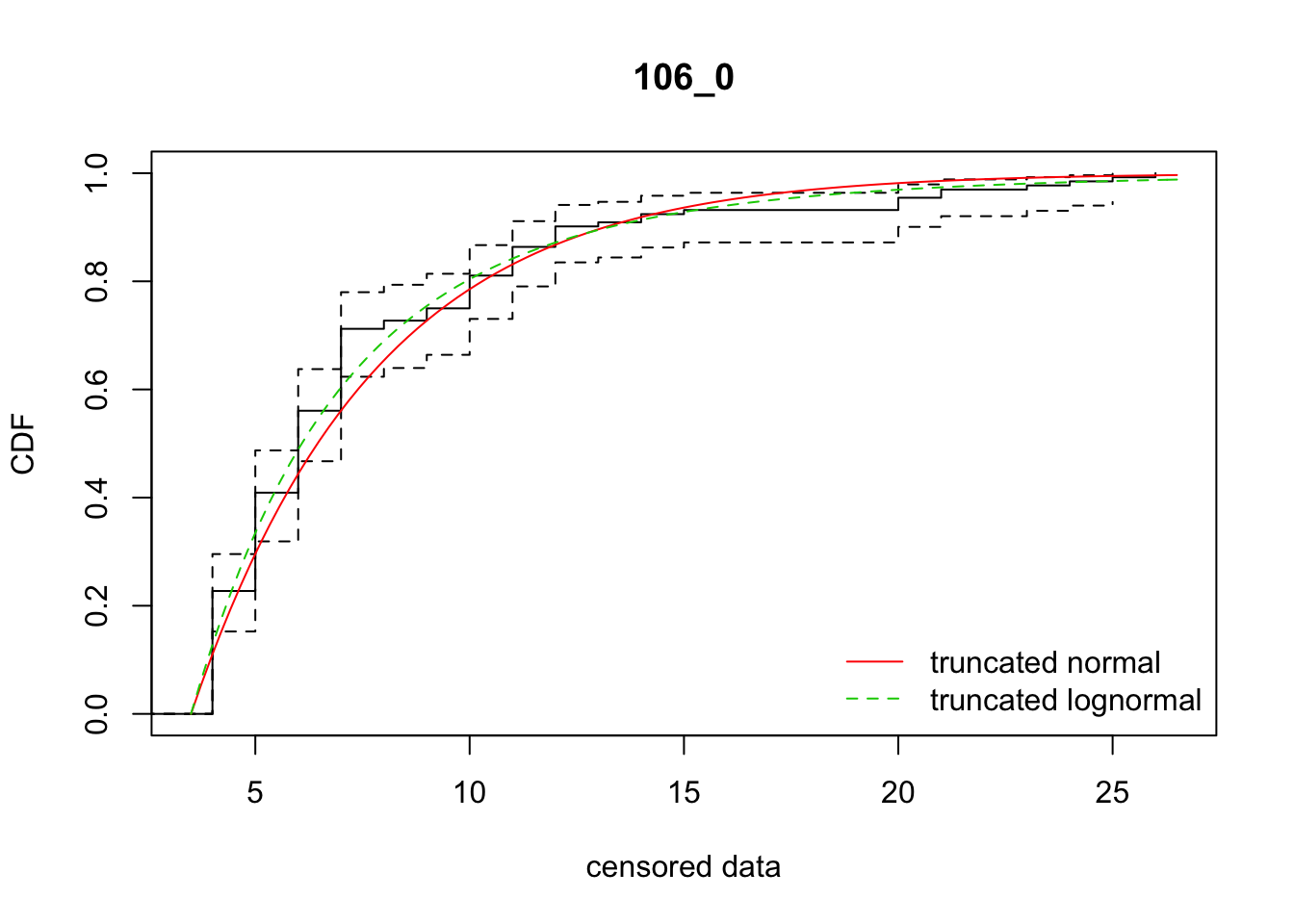
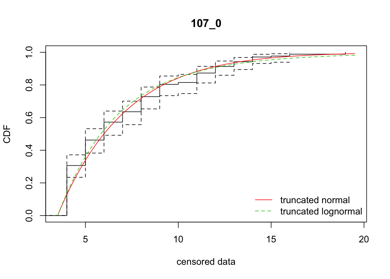
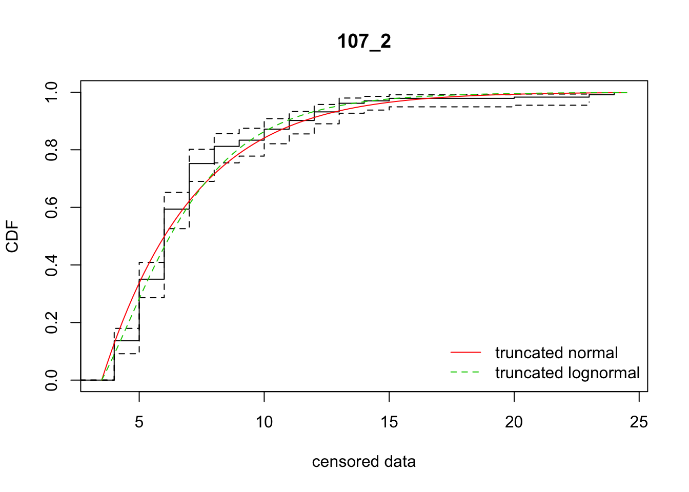
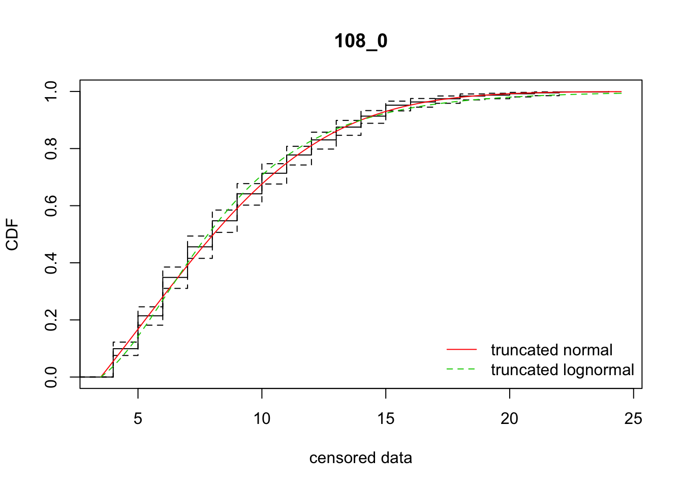
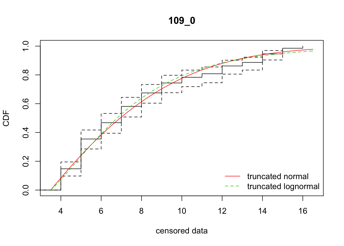
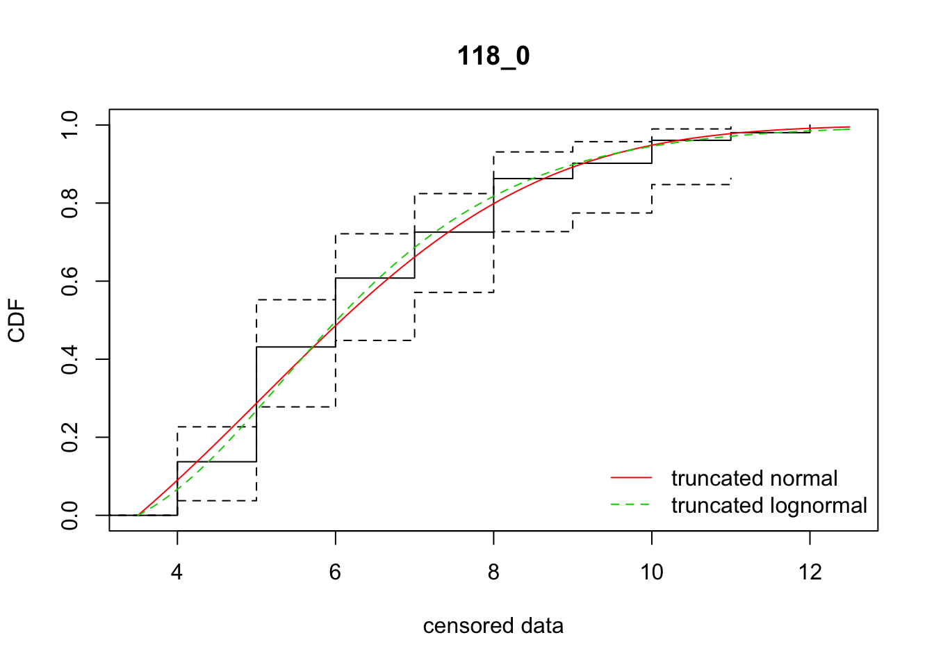
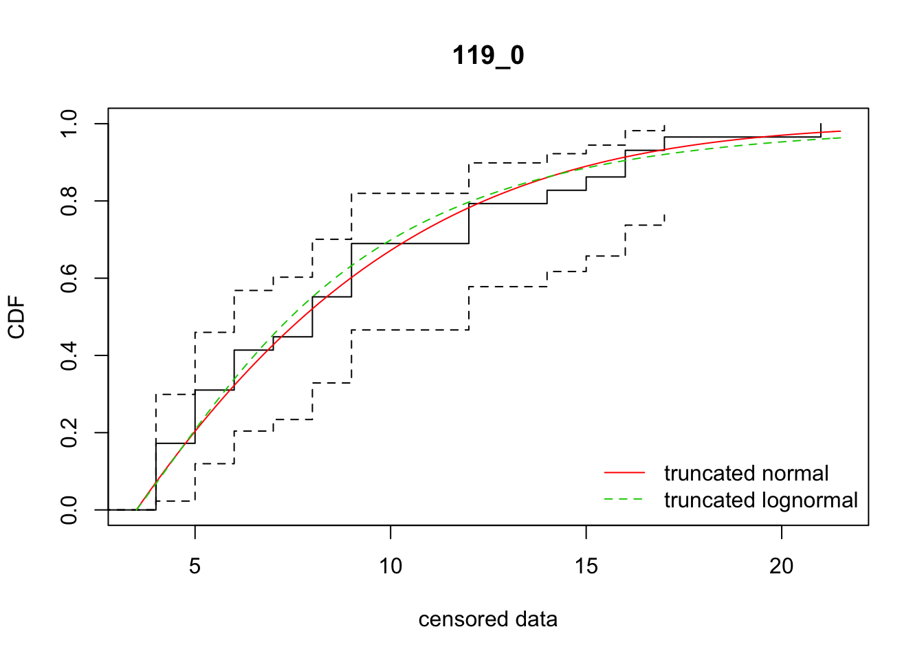
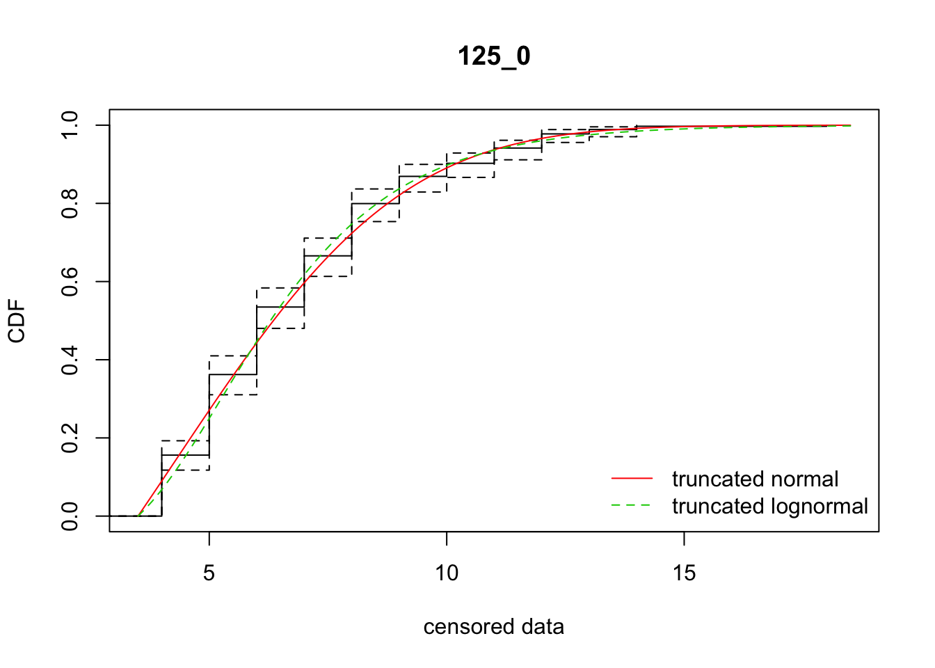
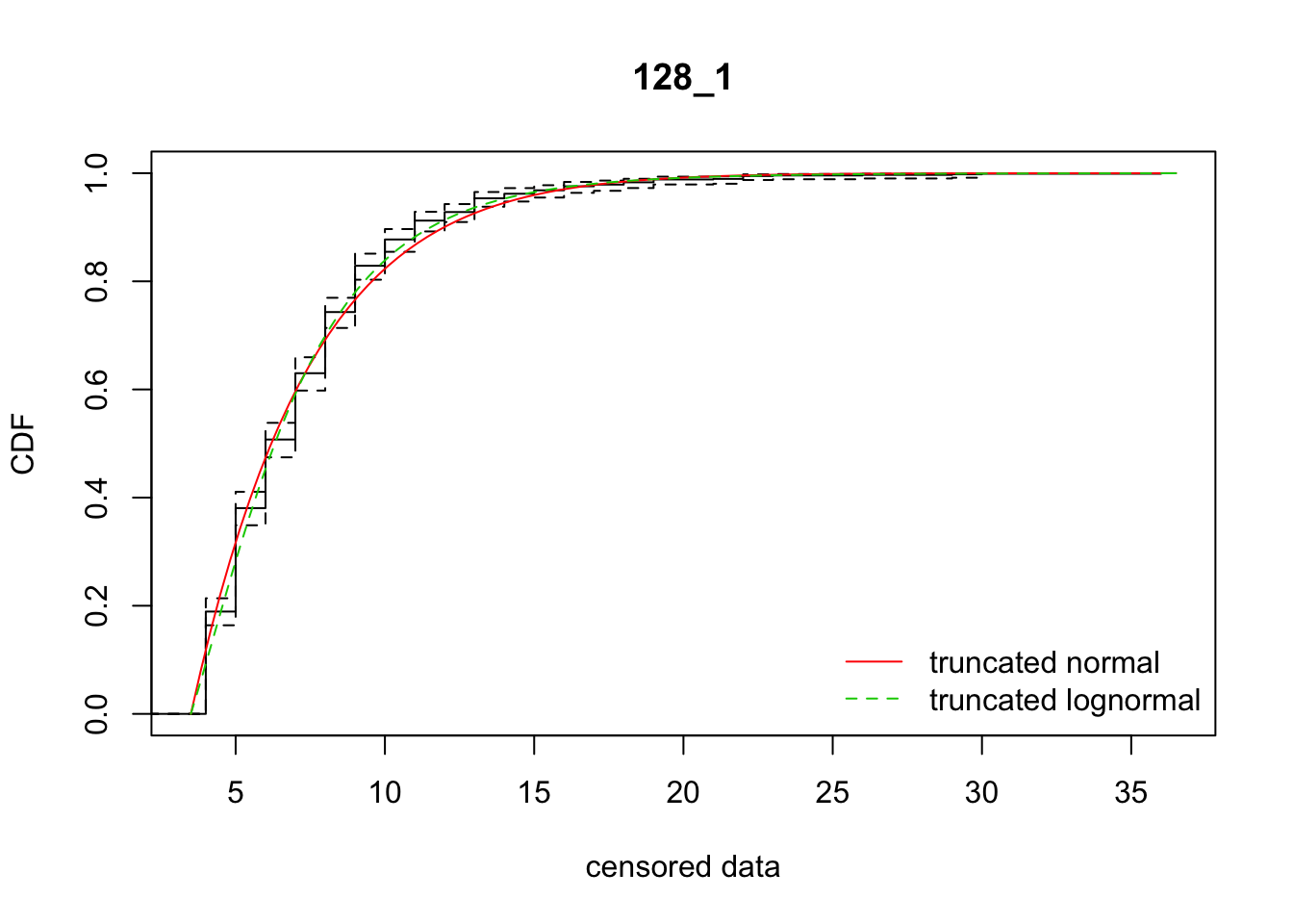
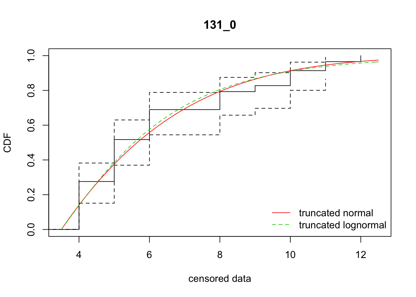
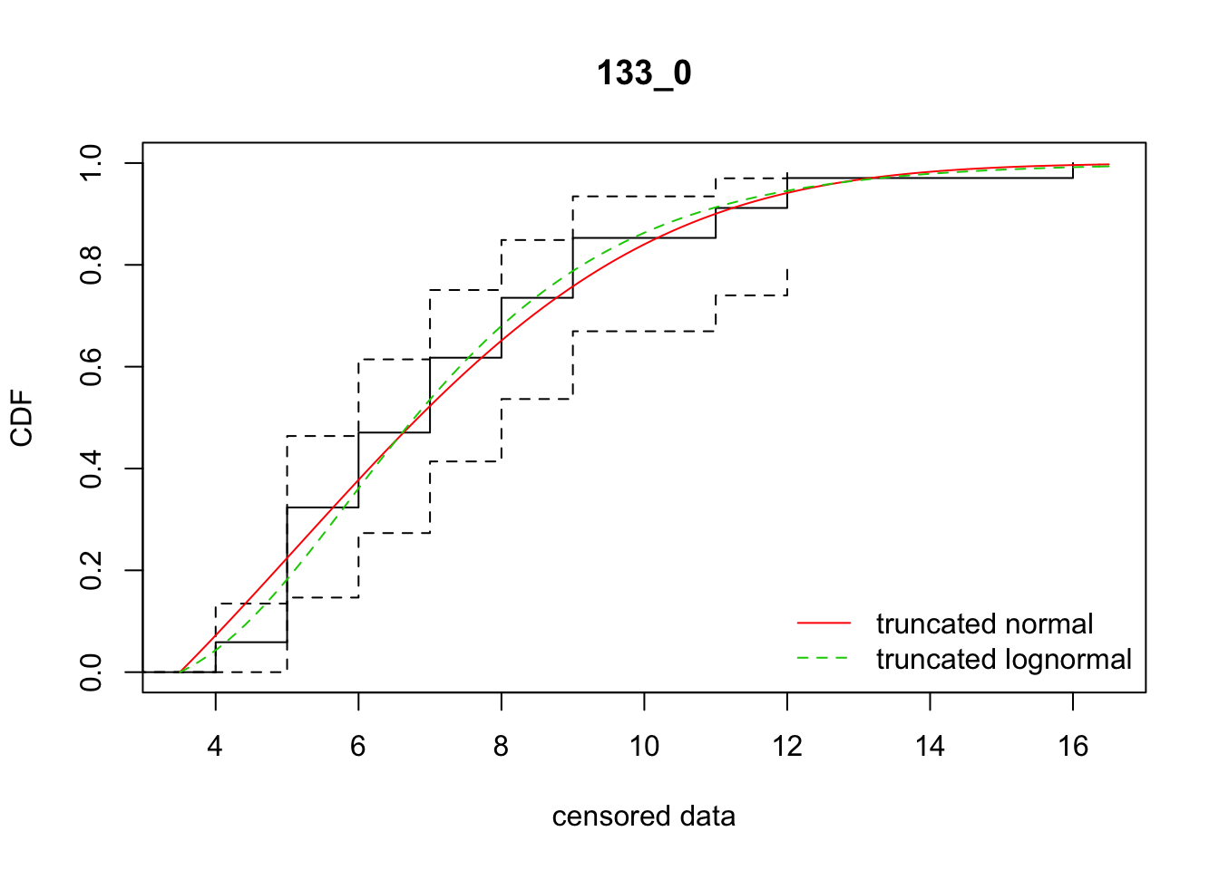
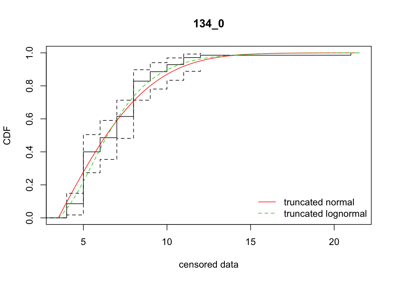
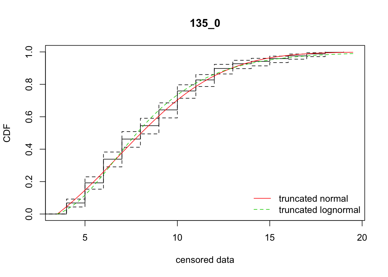
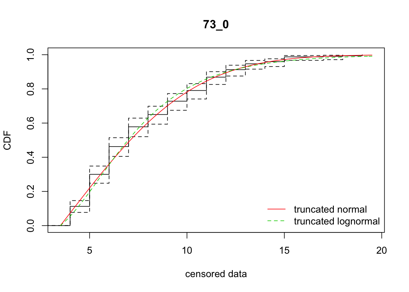
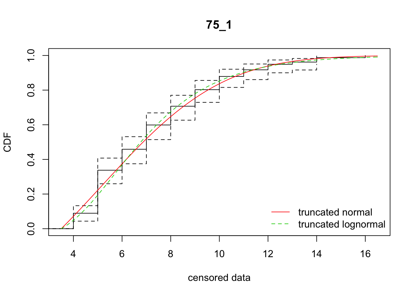
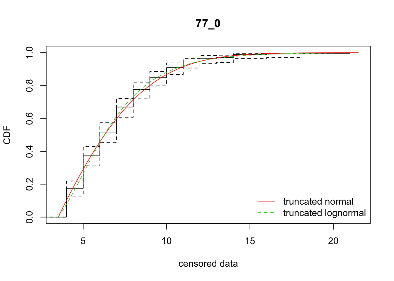
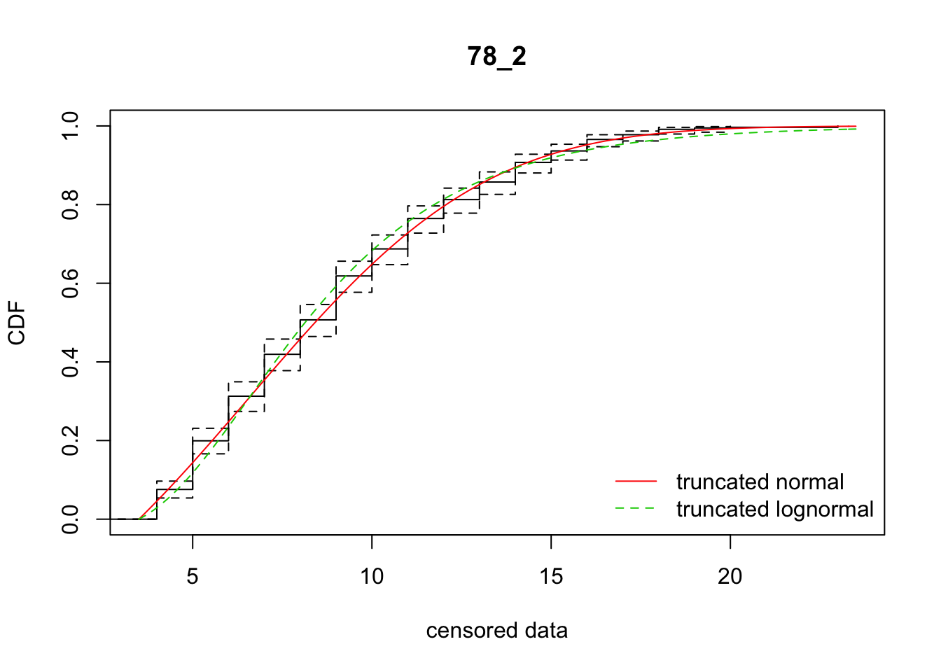
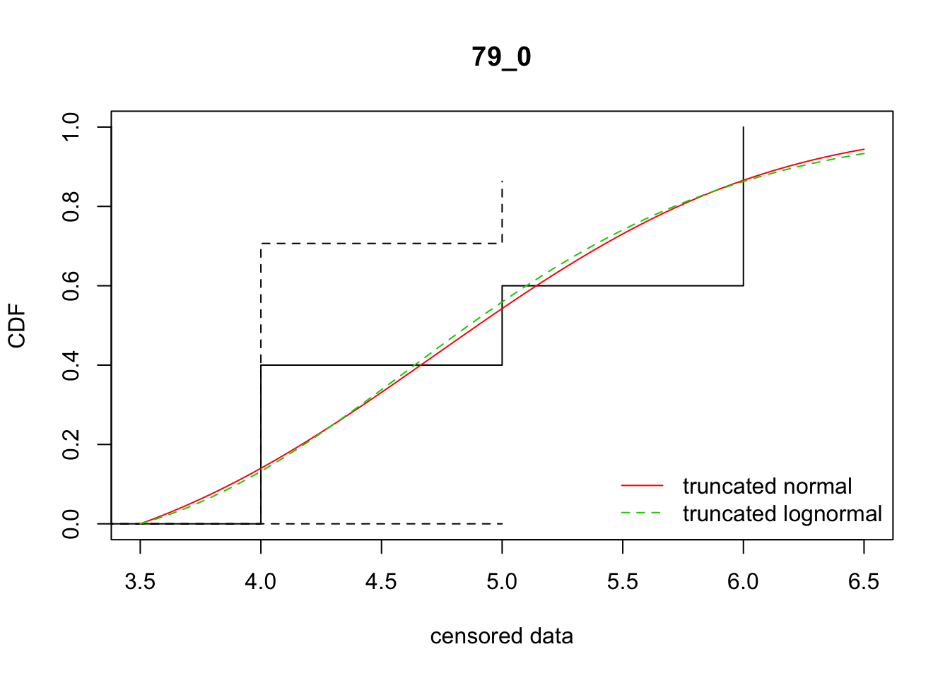
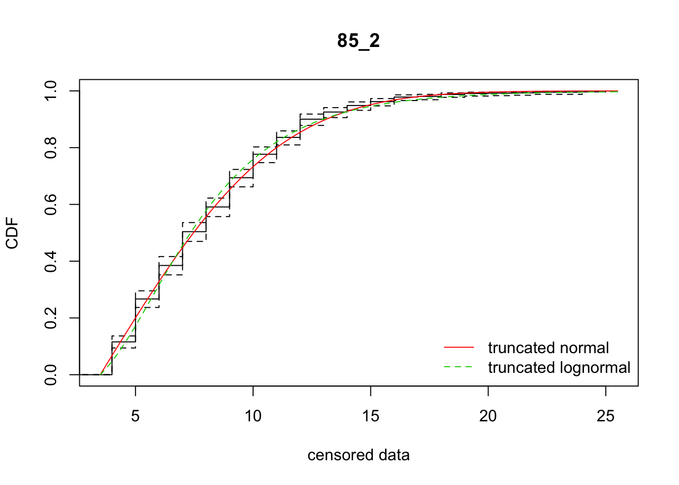
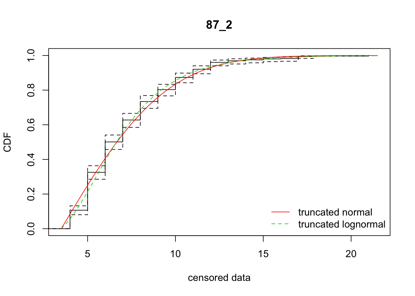
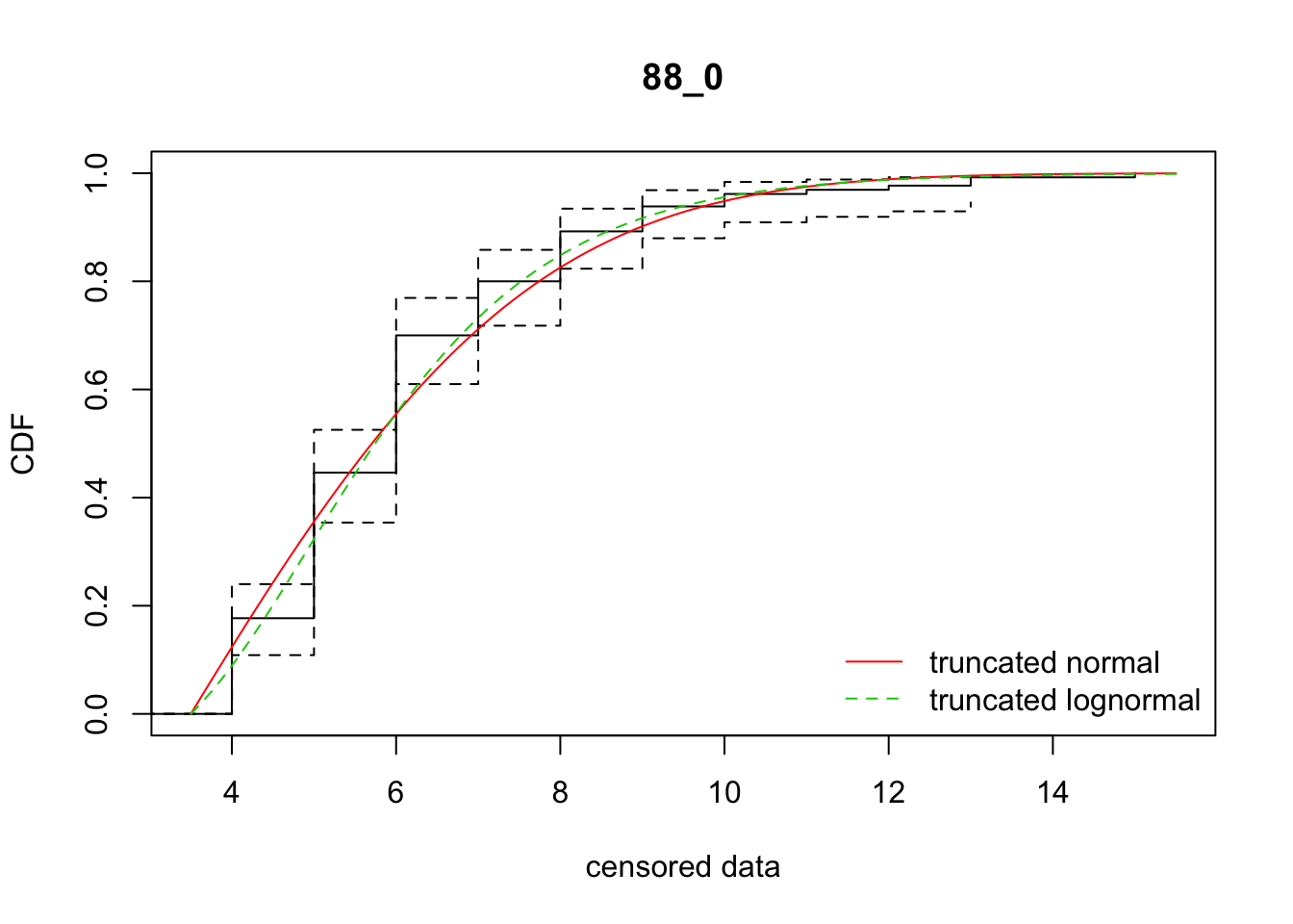
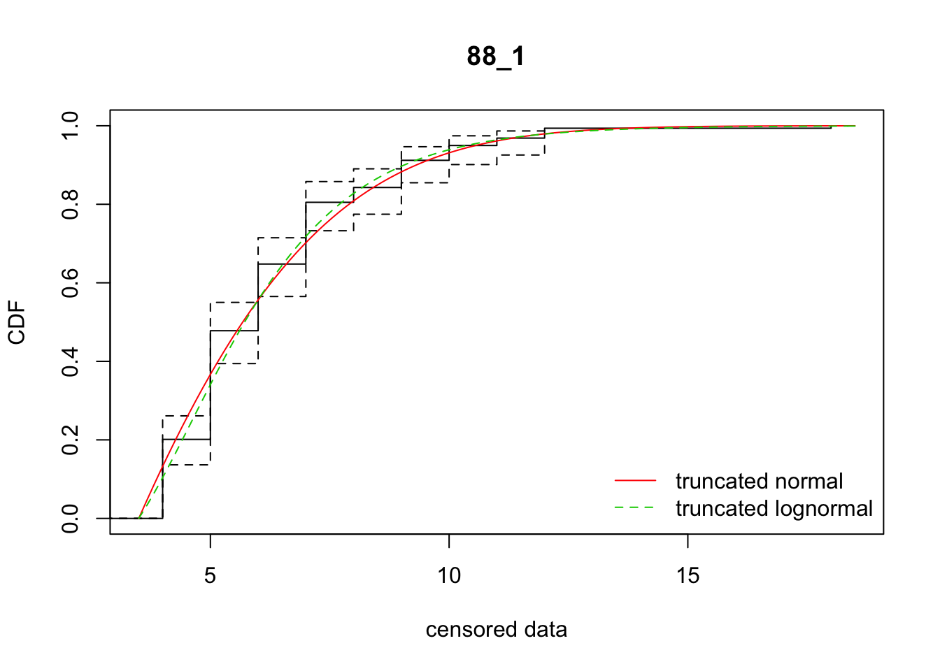
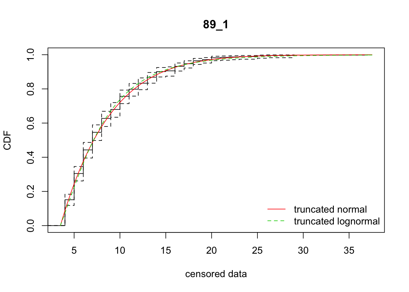
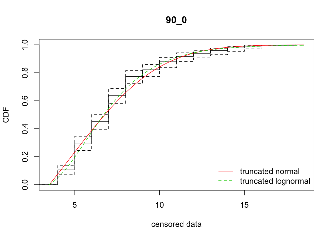
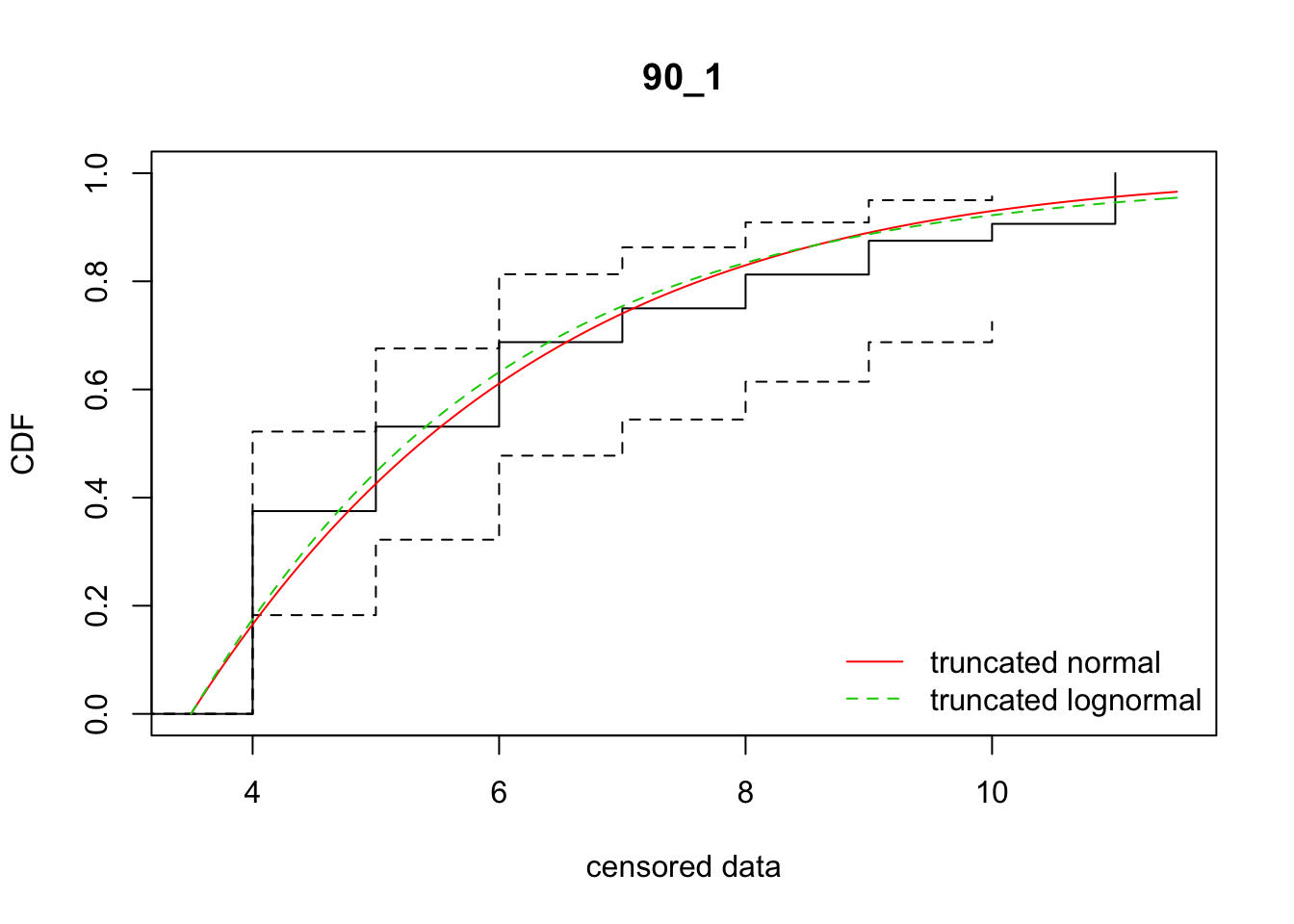
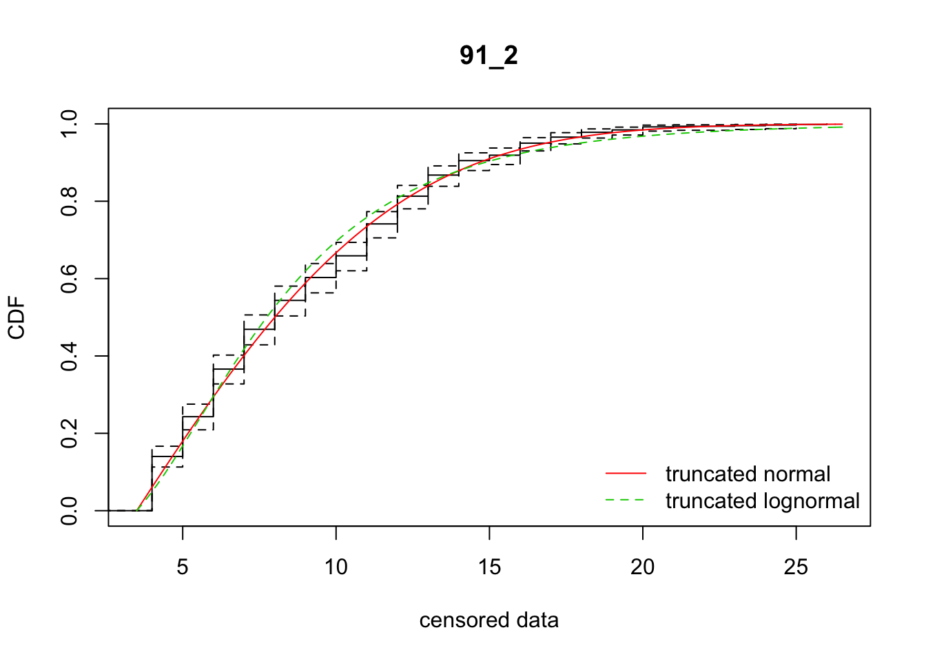
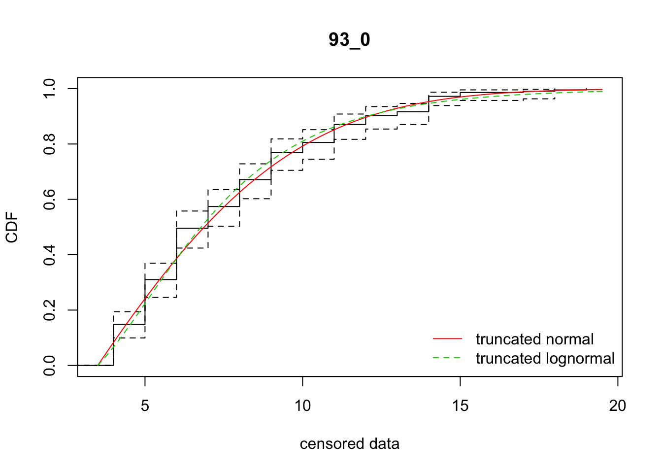
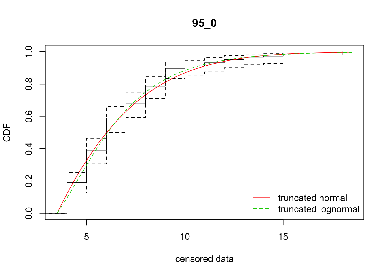
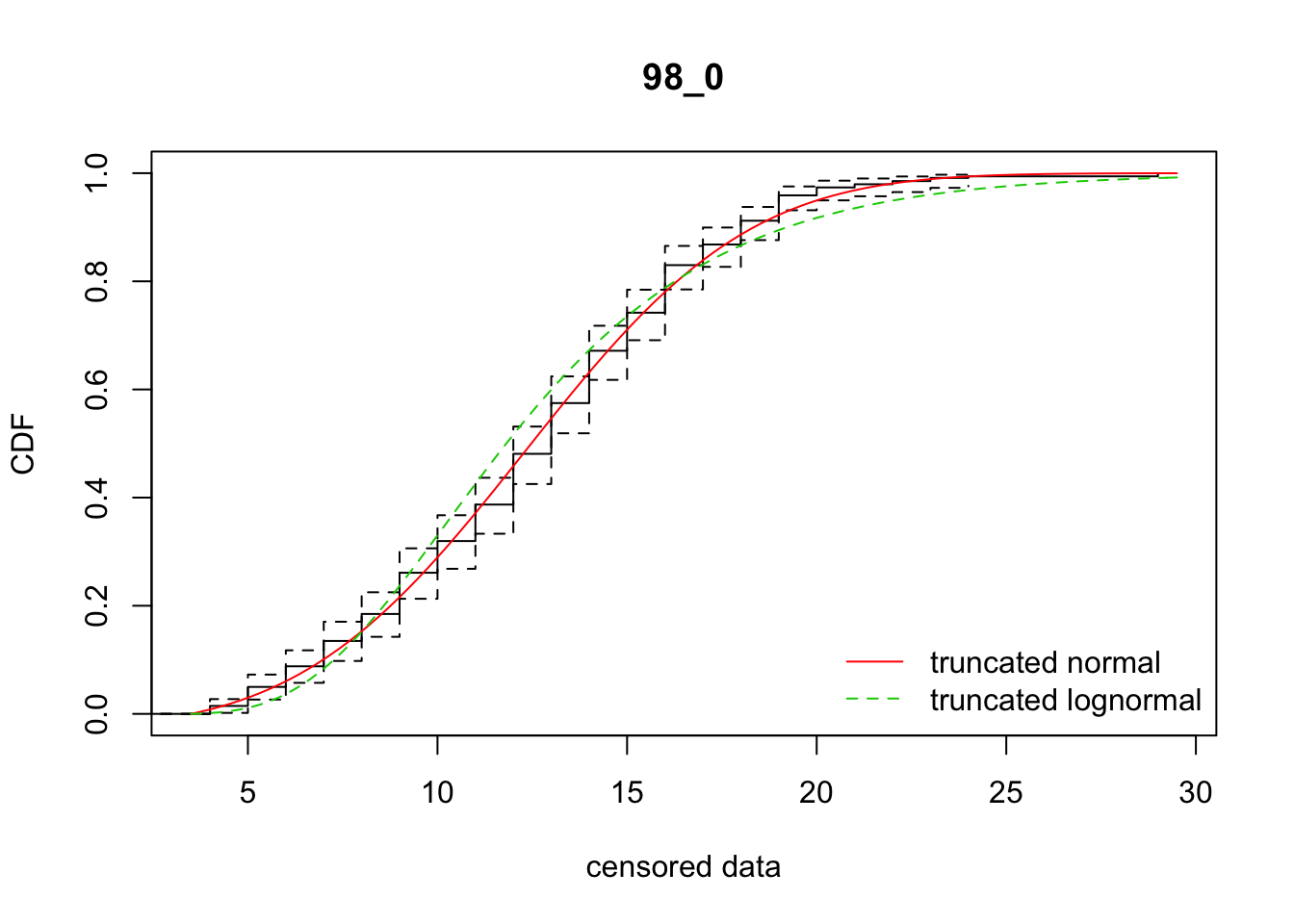
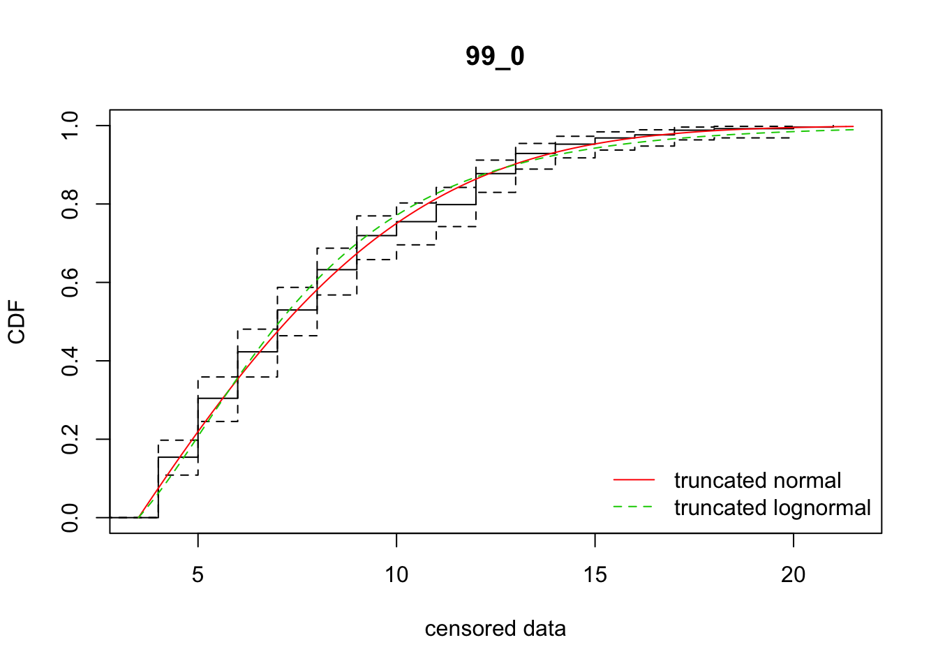
cdfcompcens(list(fit_tnorm, fit_tlnorm), Turnbull.confint = TRUE, main = dispersal_data$ID[1],
legendtext = c("truncated normal", "truncated lognormal"))
stnorm <- summary(fit_tnorm)
stlnorm <- summary(fit_tlnorm)
data.frame(ID = dispersal_data$ID[1], AICnorm = stnorm$aic, AIClnorm = stlnorm$aic,
mu = stnorm$est[1], sd = stnorm$est[2],
mulog = stlnorm$est[1], sdlog = stlnorm$est[2])
}Test it out:
fit_dispersal_models(subset(disperseLer, ID == "87_0")) 
       ID  AICnorm AIClnorm       mu       sd    mulog     sdlog
mean 87_0 2489.106 2512.976 7.681504 5.588817 2.173721 0.4584419
ddply(subset(disperseLer, ID == "87_0" | ID == "128_1"), "ID",
fit_dispersal_models)

     ID  AICnorm AIClnorm         mu        sd    mulog     sdlog
1 128_1 4388.528 4368.020 -41.254702 13.903769 1.723583 0.5179114
2  87_0 2489.106 2512.976   7.681504  5.588817 2.173721 0.4584419
Full run
all_Ler_fits <- ddply(disperseLer, "ID", fit_dispersal_models) 
Warning in sqrt(diag(varcovar)): NaNs producedWarning in sqrt(1/diag(V)): NaNs producedWarning in cov2cor(varcovar): diag(.) had 0 or NA entries; non-finite
result is doubtful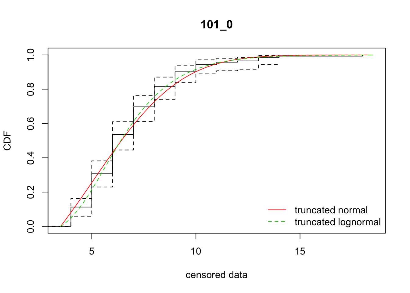


all_Ler_fits ID AICnorm AIClnorm mu sd mulog sdlog
1 100_0 210.19617 209.46451 4.0982669 2.598637 1.662753 0.3158626
2 101_0 602.77572 592.94699 5.1014741 3.277311 1.839458 0.3314258
3 104_0 3917.28412 3922.72793 -66.0205798 19.643467 1.781924 0.6310585
4 105_0 1749.42577 1745.88089 4.3716320 3.528681 1.788268 0.3682102
5 106_0 646.69449 643.17978 -207.7151988 30.384323 1.307769 0.7884596
6 107_0 785.44720 789.47637 -69.4381348 16.731328 1.359045 0.6932002
7 107_2 1063.19962 1049.11621 -70.4622184 16.881924 1.740646 0.4708113
8 108_0 3238.39521 3253.82893 5.1491554 5.733904 2.030345 0.4653378
9 109_0 986.23168 993.20962 0.3779014 6.555358 1.830760 0.5150772
10 118_0 204.70929 204.18931 5.0644220 2.761443 1.771622 0.3257241
11 119_0 159.50334 161.20702 -6.3007402 10.223254 1.877411 0.6364096
12 125_0 1535.73278 1535.21286 4.3296332 3.730306 1.802977 0.3811286
13 128_1 4388.52816 4368.01998 -41.2547017 13.903769 1.723583 0.5179114
14 131_0 238.69069 240.39449 -4.1084462 5.925933 1.515535 0.5133134
15 133_0 157.21511 155.12266 5.1511826 3.886229 1.897703 0.3621337
16 134_0 309.97239 302.59321 3.1582072 4.429201 1.839981 0.3572949
17 135_0 2047.52526 2051.75059 6.8726239 4.285294 2.044296 0.3991739
18 73_0 1532.73721 1536.47422 3.8581071 5.121355 1.901724 0.4439891
19 75_0 1268.28878 1260.59024 4.1641279 5.606950 1.984015 0.4344484
20 75_1 713.93094 712.15268 5.1754515 3.910981 1.888703 0.3829246
21 77_0 1155.49401 1152.37149 1.9264317 4.898033 1.780264 0.4203578
22 78_2 3036.48468 3056.08625 6.5758420 5.186990 2.078296 0.4447256
23 79_0 16.43216 16.74522 4.7295954 1.069369 1.567024 0.1989932
24 85_1 732.95641 721.38097 2.8431735 4.174413 1.781615 0.3625076
25 85_2 4355.97098 4360.51040 3.7176899 5.757882 1.957874 0.4585569
26 87_0 2489.10649 2512.97557 7.6815043 5.588817 2.173721 0.4584419
27 87_1 4843.91681 4931.83322 8.2138623 4.811877 2.161850 0.4406535
28 87_2 2518.89435 2497.62958 3.4870029 4.699188 1.861861 0.4004055
29 88_0 505.51054 498.61356 3.1493213 3.455050 1.709980 0.3395724
30 88_1 632.33299 627.93489 0.9579404 4.372635 1.677200 0.3862587
31 89_1 2374.42168 2376.20474 -34.9798971 15.374743 1.835881 0.6015254
32 90_0 1414.00768 1402.33081 4.8038650 4.040552 1.881511 0.3774301
33 90_1 127.58152 128.43750 -14.7687132 7.623299 1.276556 0.5866747
34 91_2 3391.73490 3426.96778 2.8737605 7.010140 1.991896 0.5304049
35 93_0 1029.93150 1033.78692 2.0282346 5.749507 1.853023 0.4719776
36 95_0 639.50220 636.32519 -4.6097825 6.728016 1.717181 0.4532293
37 98_0 1956.80573 1995.93158 12.3030722 4.651470 2.468955 0.3797439
38 99_0 1252.70855 1262.56877 2.1108985 6.230271 1.889331 0.5023501Some AIC stats
sum(all_Ler_fits$AICnorm)[1] 58230.28sum(all_Ler_fits$AIClnorm)[1] 58366.17cbind(all_Ler_fits$ID, all_Ler_fits$AICnorm - all_Ler_fits$AIClnorm) [,1] [,2]
[1,] 1 0.7316622
[2,] 2 9.8287266
[3,] 3 -5.4438047
[4,] 4 3.5448752
[5,] 5 3.5147126
[6,] 6 -4.0291707
[7,] 7 14.0834126
[8,] 8 -15.4337230
[9,] 9 -6.9779437
[10,] 10 0.5199870
[11,] 11 -1.7036794
[12,] 12 0.5199187
[13,] 13 20.5081874
[14,] 14 -1.7037993
[15,] 15 2.0924486
[16,] 16 7.3791782
[17,] 17 -4.2253246
[18,] 18 -3.7370105
[19,] 19 7.6985462
[20,] 20 1.7782603
[21,] 21 3.1225217
[22,] 22 -19.6015753
[23,] 23 -0.3130643
[24,] 24 11.5754364
[25,] 25 -4.5394237
[26,] 26 -23.8690776
[27,] 27 -87.9164058
[28,] 28 21.2647714
[29,] 29 6.8969805
[30,] 30 4.3980948
[31,] 31 -1.7830564
[32,] 32 11.6768719
[33,] 33 -0.8559744
[34,] 34 -35.2328843
[35,] 35 -3.8554141
[36,] 36 3.1770114
[37,] 37 -39.1258517
[38,] 38 -9.8602207So there’s variation among reps on which model fits better. In sum, the normal distribution is better. However, the parameter estimates are much more variable, in ways that really don’t make sense biologically, unless there is directionally biased dispersal that varies from rep to rep.