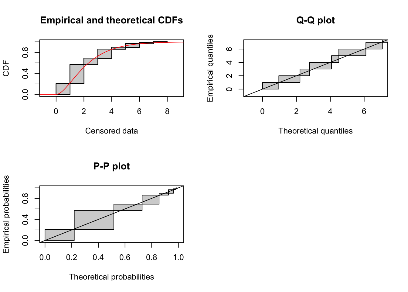
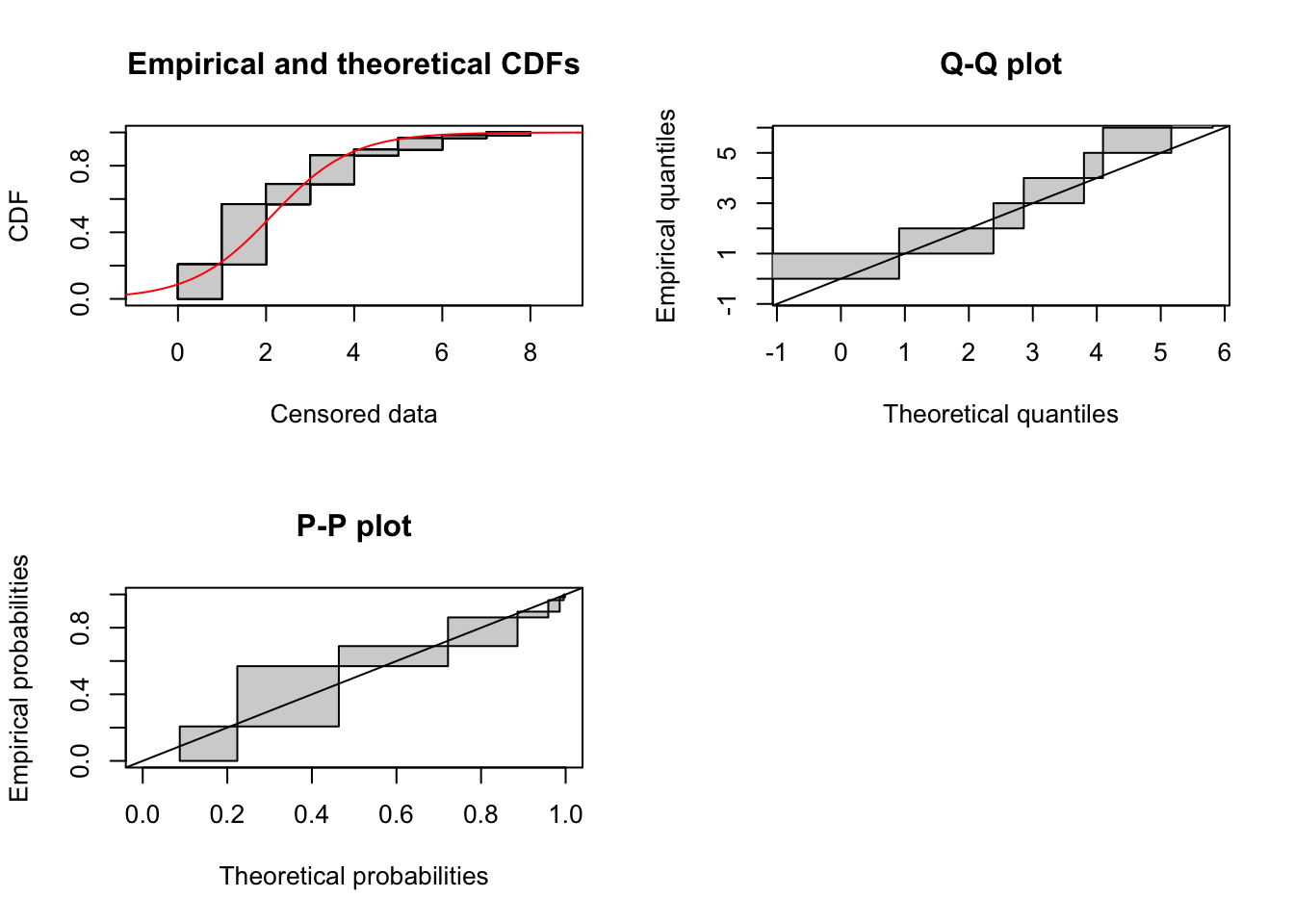
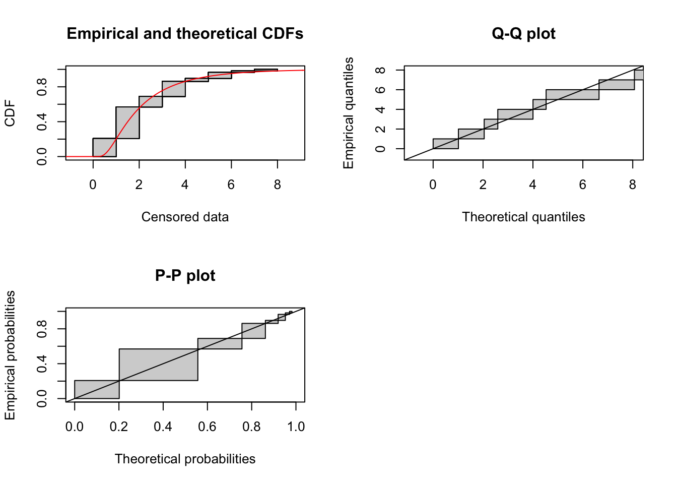
Likely-looking distributions - Project notebook for the Invasion Heterogeneity project

Let’s think about which distributions could be good. We know what the (half-)normal, exponential, and log-normal look like.

Nathan et al. (2012) also suggest:

Exponential power
2Dt
Inverse power
Logistic
Mixture models
Inverse Gaussian (Wald)
Wiebull
Gamma

The scaling factors in Nathan et al. are for two-dimensional dispersal expressed in radial distance (I think). They suggest that this can be converted to a “distance kernel” by multiplying by \(2\pi r\), but that doesn’t seem right for e.g. their Gaussian formulation.

Some notes:

Gamma is generalization of exponential. It can have a mode at the origin or at positive values. Good candidate.
Inverse Gaussian is also a good candidate, based on shape.
Both gamma and inverse Gaussian are special cases of the 3-parameter generalized inverse Gaussian. GIGrvg::(d)gig (but no p form); rmutil::(d)ginvgauss
The exponential, Weibull, and gamma are all special cases of the 3-parameter generalized gamma distribution. At least for the plots shown on wikipedia, it does not appear to allow a mode away from zero(?). flexsurv::dgengamma

Here is the list of distributions for which start values are found automatically from the help for mledist): For the following named distributions, reasonable starting values will be computed if start is omitted (i.e. NULL) : “norm”, “lnorm”, “exp” and “pois”, “cauchy”, “gamma”, “logis”, “nbinom” (parametrized by mu and size), “geom”, “beta”, “weibull” from the stats package; “invgamma”, “llogis”, “invweibull”, “pareto1”, “pareto”, “lgamma”, “trgamma”, “invtrgamma” from the actuar package.

Let’s look at some of these, with one of the datasets. We’ll start with the origin at the leading edge of the home pot, so I don’t have to deal with the left-truncation (I have an idea for generalizing that code).

temp <- filter(disperseLer, ID == "100_0")
cens_data <- cens_dispersal_data(temp, 7)

Gamma distribution

fit_gamma <- fitdistcens(cens_data, "gamma")
summary(fit_gamma)

Fitting of the distribution ' gamma ' By maximum likelihood on censored data 
Parameters
       estimate Std. Error
shape 1.9355007  0.4065521
rate  0.8327602  0.1888287
Loglikelihood:  -102.311   AIC:  208.622   BIC:  212.7429 
Correlation matrix:
          shape      rate
shape 1.0000000 0.9065196
rate  0.9065196 1.0000000

plot(fit_gamma)

Logistic distribution

fit_logis <- fitdistcens(cens_data, "logis")
summary(fit_logis)

Fitting of the distribution ' logis ' By maximum likelihood on censored data 
Parameters
          estimate Std. Error
location 2.1323049  0.2119352
scale    0.9098716  0.1028623
Loglikelihood:  -111.5651   AIC:  227.1303   BIC:  231.2511 
Correlation matrix:
           location      scale
location 1.00000000 0.09289735
scale    0.09289735 1.00000000

plot(fit_logis)

It looks like this distribution is not restricted to postive values, so needs to be truncated anyway. It seems unlikely to be a good generic fit as it never allows a mode away from zero (just a plateau).

Weibull distribution

fit_weibull <- fitdistcens(cens_data, "weibull")
summary(fit_weibull)

Fitting of the distribution ' weibull ' By maximum likelihood on censored data 
Parameters
      estimate Std. Error
shape 1.427613  0.1622270
scale 2.554287  0.2546927
Loglikelihood:  -102.4526   AIC:  208.9051   BIC:  213.026 
Correlation matrix:
          shape     scale
shape 1.0000000 0.3598061
scale 0.3598061 1.0000000

plot(fit_weibull)

Inverse Gaussian

This requires setting start values to the parameters. Following the logic of other functions in fitdistrplus, we’d like to match empirical moments. Wikipedia (https://en.wikipedia.org/wiki/Inverse_Gaussian_distribution) gives a distribution in terms of \(\mu\) and \(\lambda\), where the mean is \(\mu\) and the variance is \(\mu^3/\lambda\). The function in actuar has parameters “mean” and “shape.” It is described in terms of of the “dispersion” parameter which is the inverse of shape; inspection reveals that “mean” is \(\mu\) and “dispersion” is \(1/\lambda\) in the Wikipedia formulation, so “shape” is \(\lambda\). Thus we want to estimate start values using mean = mean(x) and shape = mean(x)^3 / var(x).

library(actuar)
x <- apply(cens_data, 1, mean) # set each value to the middle of its interval
start_pars <- list (
                      mean = mean(x),
                      shape = mean(x)^3 / var(x)
                    )
fit_invgauss <- fitdistcens(cens_data, "invgauss", start = start_pars)

Warning in checkparamlist(arg_startfix$start.arg, arg_startfix$fix.arg, :
Some parameter names have no starting/fixed value but have a default value.

summary(fit_invgauss)

Fitting of the distribution ' invgauss ' By maximum likelihood on censored data 
Parameters
      estimate Std. Error
mean  2.339617  0.2437156
shape 3.804128  0.8686025
Loglikelihood:  -102.5821   AIC:  209.1642   BIC:  213.285 
Correlation matrix:
            mean      shape
mean  1.00000000 0.03855307
shape 0.03855307 1.00000000

plot(fit_invgauss)

I’ve created a function start_params() in helpers.R that does this:

function (x, dist) 
{
    if (dim(as.matrix(x))[2] == 2) {
        x <- apply(x, 1, mean)
    }
    else if (dim(as.matrix(x))[2] > 2) {
        stop("x must be a vector or two-column matrix")
    }
    start_pars <- switch(dist, invgauss = list(mean = mean(x), 
        shape = mean(x)^3/var(x)), NULL)
    if (is.null(start_pars)) {
        warning("No method exists for setting start values for ", 
            dist)
    }
    return(start_pars)
}

I will add other distributions in the switch function. Here’s a test that it works:

library(actuar)
start_pars <- start_params(cens_data, "invgauss")
fit_invgauss <- fitdistcens(cens_data, "invgauss", start = start_pars)

Warning in checkparamlist(arg_startfix$start.arg, arg_startfix$fix.arg, :
Some parameter names have no starting/fixed value but have a default value:
dispersion.

summary(fit_invgauss)

Fitting of the distribution ' invgauss ' By maximum likelihood on censored data 
Parameters
      estimate Std. Error
mean  2.339617  0.2437156
shape 3.804128  0.8686025
Loglikelihood:  -102.5821   AIC:  209.1642   BIC:  213.285 
Correlation matrix:
            mean      shape
mean  1.00000000 0.03855307
shape 0.03855307 1.00000000

Generalized gamma distribution

This is provided by flexsurv, with root gengamma. This implementation has parameters \(\mu\), \(\sigma\), and \(Q\).

The Wikipedia definition (https://en.wikipedia.org/wiki/Generalized_gamma_distribution) is \[ f(x | a, d, p) = \frac{(p/a^d)x^{d -1}e^{-(x/a)^p}}{\Gamma(d/p)} \] The Wikipedia article includes the conversion to the flexsurv definition: \[ \begin{aligned} \mu &= \ln a + \frac{\ln d - \ln p}{p}\\ \sigma &= \frac{1}{\sqrt{pd}}\\ Q &= \sqrt{p/d} \end{aligned} \] We actually need to invert these to do the substitutions in the moment calculations. We have \[ \begin{aligned} d/p &= Q^{-2}\\ pd &= \sigma^{-2}\\ d/p &= (\sigma p)^{-2} = Q^{-2}\\ p &= Q/\sigma\\ d &= 1/(\sigma Q)\\ \ln a &= \ln (d/p)^{-p} - \mu = \ln Q^{2 Q/\sigma} - \mu\\ a &= \exp\left[ \ln Q^{2 Q/\sigma} - \mu\right] \end{aligned} \] But actually, this isn’t going to help much, because the terms for the mean and variance on Wikipedia aren’t going to be invertible (at least not easily).

From the description on the help page, it seems like \(\mu\) is the mean of \(x\) and \(\sigma\) is the sd of \(\log(x)\). Let’s give this a try:

library(flexsurv)
x <- rgengamma(1000, 2, 3, 0)
mean(x)

[1] 469.7918

mean(log(x))

[1] 2.005169

sqrt(var(log(x)))

[1] 3.001755

When \(Q=0\) (the lognormal limit) then \(\mu\) is the mean of \(\log(x)\) and \(\sigma\) is the sd of \(\log(x)\). But the meanings are rather different at the Weibull and gamma limits, as described in the help for gengamma. So I think the strategy will be to fit those three standard parameters and use the AIC-best to set the start values for gengamma.