More on distributions

Generalized gamma

I’ve made a specialized start function for gengamma:

start_gengamma

function (x, truncated = FALSE) 
{
    if (dim(as.matrix(x))[2] != 2) {
        stop("Only interval-censored methods have been developed in start_gengamma")
    }
    dist_list <- c("lnorm", "weibull", "gamma")
    n <- length(dist_list)
    base_fits <- data.frame(dist = dist_list, AIC = numeric(n), 
        p1 = numeric(n), p2 = numeric(n), stringsAsFactors = FALSE)
    base_starts <- array(list(NULL), n)
    if (truncated) {
        stop("Truncated methods have not yet been developed in start_gengamma")
    }
    for (i in 1:n) {
        fit <- fitdistcens(x, base_fits$dist[i], base_starts[[i]])
        base_fits$AIC[i] <- fit$aic
        base_fits$p1[i] <- coef(fit)[1]
        base_fits$p2[i] <- coef(fit)[2]
    }
    best <- base_fits[which.min(base_fits$AIC), ]
    start_pars <- with(best, switch(dist, lnorm = list(mu = p1, 
        sigma = p2, Q = 2), weibull = list(mu = log(p1), sigma = 1/p2, 
        Q = 1), gamma = list(mu = log(p1/p2), sigma = sqrt(1/p1), 
        Q = sqrt(1/p1))))
    return(start_pars)
}

This can called via start_params():

start_params

function (x, dist, ...) 
{
    x_orig <- x
    if (dim(as.matrix(x))[2] == 2) {
        x <- apply(x, 1, mean)
    }
    else if (dim(as.matrix(x))[2] > 2) {
        stop("x must be a vector or two-column matrix")
    }
    start_pars <- switch(dist, invgauss = list(mean = mean(x), 
        shape = mean(x)^3/var(x)), gengamma = start_gengamma(x_orig, 
        ...), NULL)
    if (is.null(start_pars)) {
        warning("No method exists for setting start values for ", 
            dist)
    }
    return(start_pars)
}

Note that the optional parameter truncated can be passed through via the dots. The truncated case needs to be written (the function in fitdistcens will be different).

Note that there are comments in the code that are not coming through here—somehow the rmarkdown rendering is “tidying” the code output!

Exponential power

This is another name for the generalized normal (https://en.wikipedia.org/wiki/Generalized_normal_distribution) and has been implemented in package gnorm (https://cran.r-project.org/web/packages/gnorm/vignettes/gnormUse.html). It’s a three-parameter distribution with the normal, Laplace and uniform distributions as special cases. It’s defined on the whole real line, so I could either truncate it (allowing the mode to be either positive or negative) or make a “half-gnorm,” setting the location parameter (mu) at zero and reflecting the distribution.

Getting start values for the parameters is non-trivial (the Gamma function would need to be inverted!), but a decent starting place in either case would be beta = 2, which gives the normnal distribution; in that case the sigma of the normal distribution is equivalent to sqrt(2) * alpha.

Half-normal

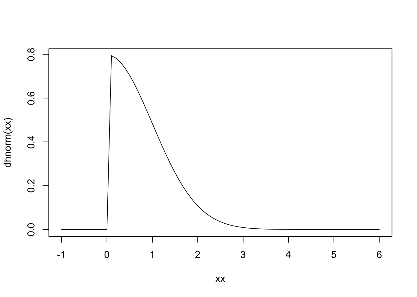
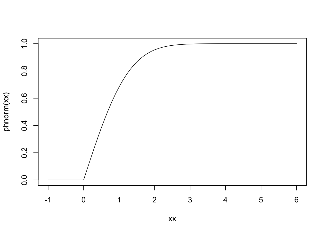
So let’s look at half-distributions (which will also be needed for 2Dt). Here’s what I think it would look like:

dhnorm <- function(x, sigma = 1, log = FALSE) {
  (x > 0) * 2 * dnorm(x, 0, sigma, log)
}
phnorm <- function(q, sigma = 1, lower.tail = TRUE, log.p = FALSE) {
  phn <- (q > 0) * (1 - 2 * pnorm(q, 0, sigma, lower.tail = FALSE))
  if (!lower.tail) phn <- (q > 0) * (1 - phn)
  if (log.p) phn <- log(phn)
  phn
}
xx <- seq(-1, 6, 0.1)
plot(xx, dhnorm(xx), type = "l")

plot(xx, phnorm(xx), type = "l")

I’ve put the above functions in dists.R and added the distribution to start_params()

2dt distribution

The formula for the density function of the 2dt distribution given by Nathan et al. (2012) is \[ f(x; a,b) = \frac{b-1}{\pi a^2}\left( 1 + \frac{x^2}{a^2}\right)^{-b}. \] Bullock et al (2017) claim to be using Nathan’s formulations but omit the final exponent (although there’s no way of knowing whether that’s a typo in the table, as they don’t appear to provide their code): \[ f(x; a,b) = \frac{b-1}{\pi a^2}\left( 1 + \frac{x^2}{a^2}\right). \] Clark’s (1999) original formula is \[ f(x; u,p) = \frac{p}{\pi u} \left( 1 + \frac{x^2}{u}\right)^{-(p+1)}. \] This is equivalent to the Nathan formulation if we let \(b = p+1\) and \(a = \sqrt{u}\).

The Nathan formula is for what he calls \(k_L(r)\), the “location kernel.” In 2-d space (the primary focus of the paper), this will be quite different from the “distance kernel” (\(k_D(r)\)) because of the increasing area at each distance. However, in one dimension with bi-directional dispersal \(k_D(r) = 2k_L(r)\), and in fact we are measuring half of that, or \(k_L(r)\). But there are factors of \(a\) and 2 that look suspicious.

Let’s compare Nelson’s formulations with the theoretical ones for some standard distribution. We’ll start with the exponential, which in the theoretical case is only has non-negative support. The theoretical distribution is \[ f(x; \lambda) = \lambda e^{-\lambda x}. \] Nathan’s formulation is \[ f(x; a) = \frac{1}{2\pi a^2} e^{-x/a}. \] From the term in the exponential we get \(a = 1/\lambda\); but then there is an extra \(1/2\pi a\) in Norman’s normalization constant. This is different from Nathan’s claimed conversion from \(k_L(r)\) to \(k_D(r)\) in the 2D case, which is a factor of \(2 \pi x\) (although note that the distributions are formulated such that \(a = E[x]\)).

Now let’s look at the normal distribution, which has support on the full real line (as would 2Dt, as it has terms only in \(x^2\)). The theoretical distribution is \[ f(x; \mu, \sigma) = \frac{1}{\sqrt{2 \pi \sigma^2}} e^{-\frac{(x - \mu)^2}{2 \sigma^2}}. \] The half-normal is thus, for \(x \ge 0\), \[ f(x; \sigma) = \frac{2}{\sqrt{2 \pi \sigma^2}} e^{-\frac{x^2}{2 \sigma^2}}. \] Nathan’s formula is \[ f(x; a) = \frac{1}{\pi a^2} e^{-\frac{x^2}{a^2}}. \] From the term in the exponential, we get that \(a = \sqrt{2\pi \sigma^2}\), and thus the normalization term is \(\frac{1}{\sqrt{2 \pi \sigma^2}} \frac{1}{\pi a} = \frac{2}{\sqrt{2 \pi \sigma^2}} \frac{1}{2 \pi a}\). So once again we have to multiply Nelson’s form by \(2 \pi a\) to get the distribution we want.

This means that the distribution function we want for the 2Dt is \[ f(x; a,b) = \frac{2(b-1)}{a}\left( 1 + \frac{x^2}{a^2}\right)^{-b}, \] with \(x \ge 0\).

However, there does not seem to be a straightforward analytical solution to the integral of this, for calculating the CDF, which is need by fitdist (the p form of the distribution). I could make a version with numerical integration; the question is, what sort of vectorization (if any) is required by fitdist? In fact, the built-in distribution functions seem to have rather unpredictable responses if vectors are provided for both x (or q) and one or more parameters. A quick google did not pull up any description; and since they use c code it’s not easy to see what’s going on.

The numerical integration is not vectorized, I think. Furthermore, the function to be used by optim is supposed to return a scalar result, so I think that we don’t need to worry about vectorization over parameters. But there may well be vectorization over x and q. I think the approach could be to write some draft functions and include warning statements that show the the dimensions of various inputs. That’s for tomorrow.

Log-sech distribution

A quick note that the log-sech distribution was one of the best. This wasn’t on my previous list. So need to look into that. I also think that I haven’t yet delved into the inverse power distribution.