Half-normal distribution - Project notebook for the Invasion Heterogeneity project

Last year I wrote a half-normal distribution but didn’t actually test its fitness for fitting the data. So let’s try it out.

Our usual data:

temp <- filter(disperseLer, ID == "100_0")
cens_data <- cens_dispersal_data(temp, 7)

Let’s give it a try:

try(fitdistcens(cens_data, "hnorm"))

Error in computing default starting values.

Nope, it needs a start value. Fortunately I already provided one in start_params()!

try(fitdistcens(cens_data, "hnorm", start = start_params(cens_data, "hnorm")))

Fitting of the distribution ' hnorm ' on censored data by maximum likelihood 
Parameters:
      estimate
sigma 2.851693

It works!

Just out of curiousity, how good is the fit?

f1 <- fitdistcens(cens_data, "hnorm", start = start_params(cens_data, "hnorm"))
summary(f1)

Fitting of the distribution ' hnorm ' By maximum likelihood on censored data 
Parameters
      estimate Std. Error
sigma 2.851693  0.2674797
Loglikelihood:  -103.1706   AIC:  208.3412   BIC:  210.4016

try(plot(f1))

Oh dear, plotting requires that the quantile form of the distribution also be defined!

But we can get a basic plot:

try(plot(f1, NPMLE.method = "Turnbull"))

Warning in plotdistcens(censdata = x$censdata, distr = x$distname, para = c(as.list(x$estimate), : Q-Q plot and P-P plot are available only using the method implemented in the package npsurv (Wang) 
            with the arguments NPMLE.method at Wang (default recommended arguments).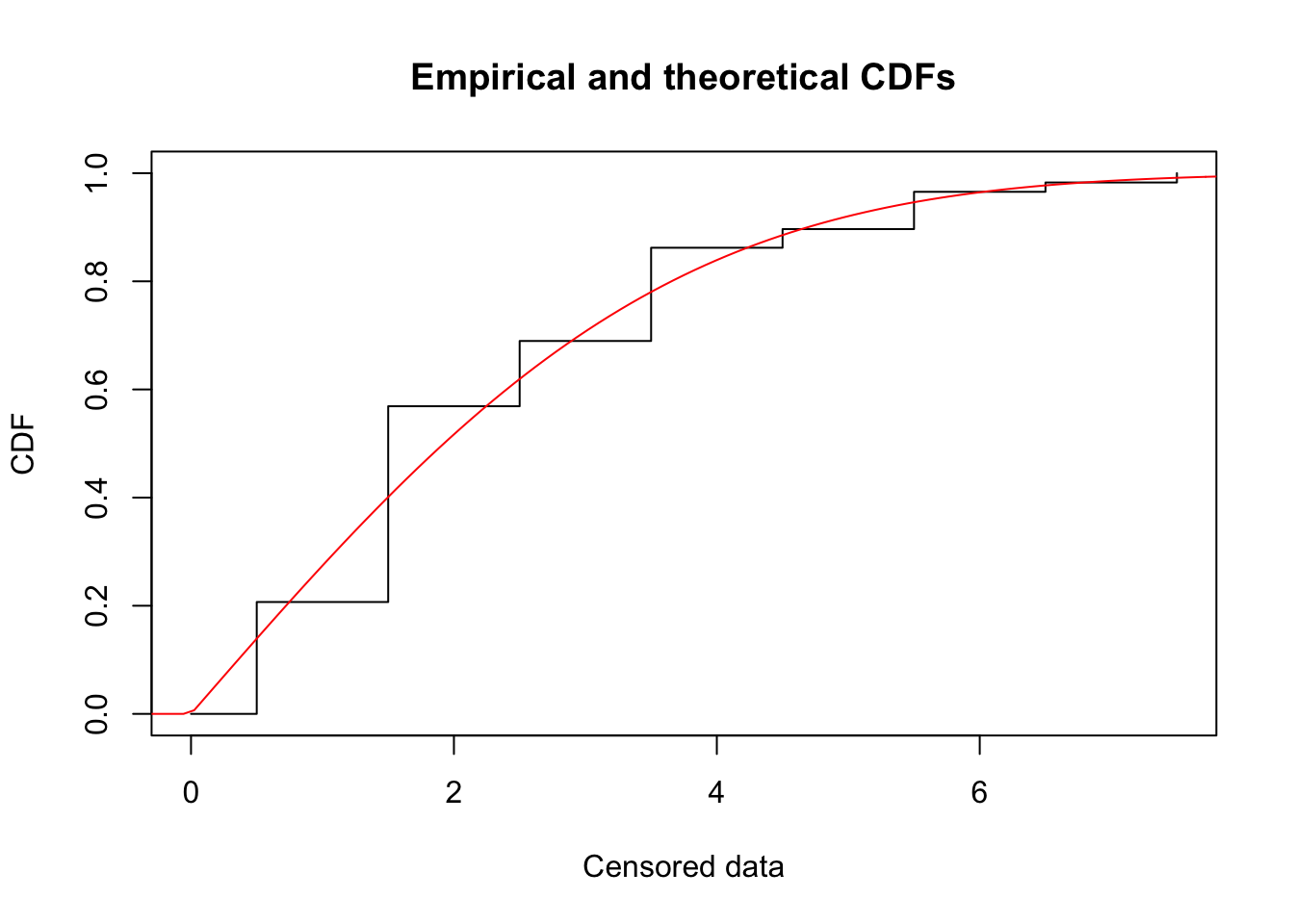

Note that, for this dataset, the AIC is about the same as for the gamma and Weibull!