Time is running short for the Davis presentation. So, at least for now, I will accept the generalized gamma distribution and the subset of data to which it fits, and move forward with creating the model.
What I need to do:
- Double check that that the replicate-specific model fits better than a single set of parameters for all the data
- Plot the resulting dispersal kernels
- Plot the patterns of covariance in parameters
- Quantify the meta-distribution of parameters, to use in the model
Evidence of heterogeneity
The replicates to which gengamma didn’t fit were 79_0 and 90_1. So drop these from the dataset:
disperseLer2 <- filter(disperseLer, ID != "79_0", ID != "90_1")Now fit the combined data:
fitall <- fit_dispersal_untruncated(disperseLer2, model = "gengamma")
fitall[, -1]
model AIC par1 par2 par3 se1 se2
1 gengamma 59533.29 1.616633 0.8058442 1.043558 0.0148677 0.007544482
se3
1 0.03199557Now fit the combined data and sum the AIC:
fiteach <- fiteach_disp_unt(disperseLer2, model = "gengamma")
sum(fiteach$AIC)
[1] 57957.58The replicate-specific fits have a cumulative AIC that is massively smaller than the fit to the lumped data (by 1576 AIC units!), so we are safe to assume heterogeneity among replicates.
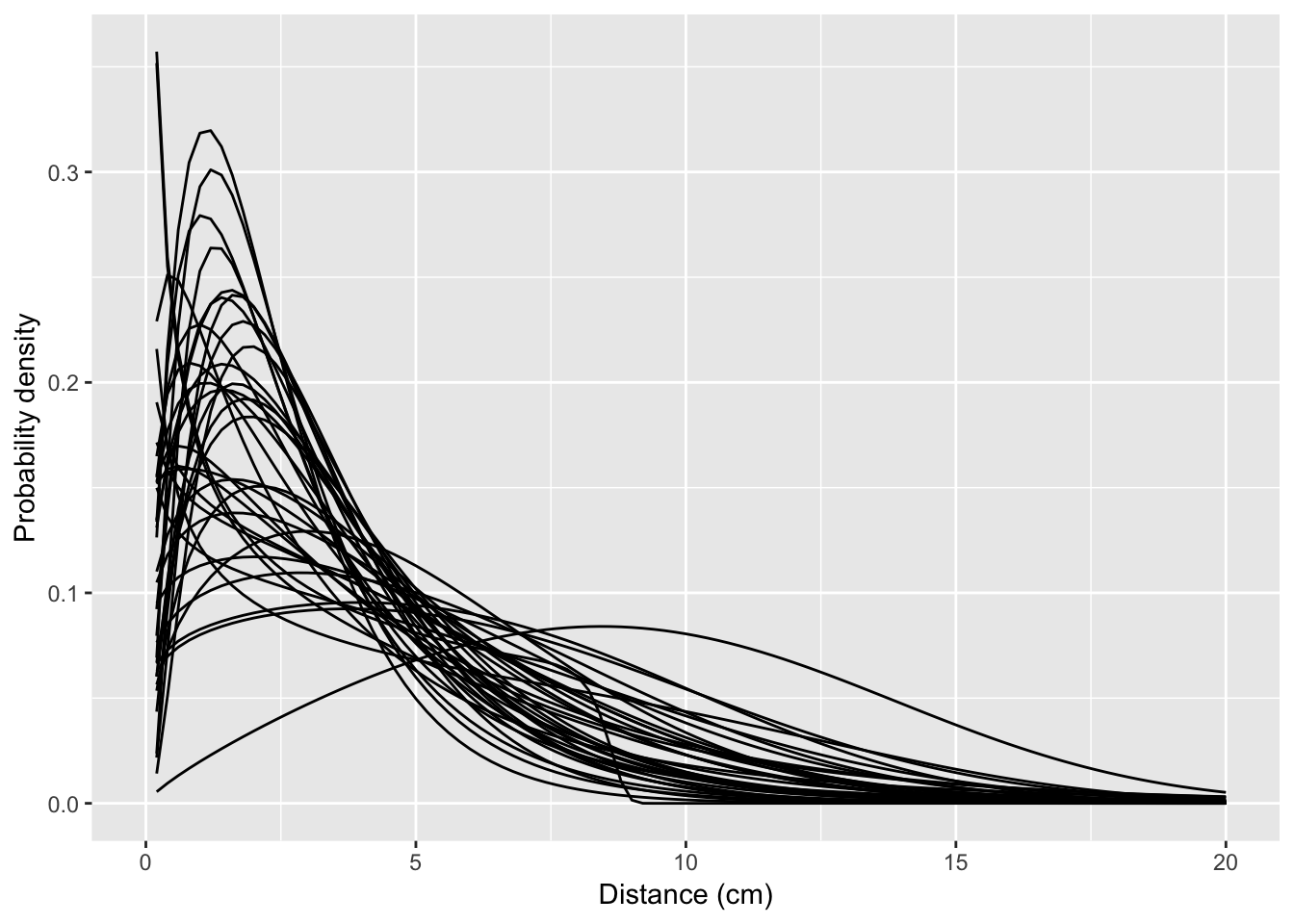
Plotting the kernels
Unfortunately, it does not appear that stat_function() in ggplot2 has a straightforward way of iteratively building functions from a table of parameters. So let’s try a loop:
p <- ggplot(data = data.frame(x = c(0, 20)), mapping = aes(x = x))
for (i in 1:nrow(fiteach)) {
  pvec <- as.numeric(fiteach[i, 4:6])
  plist <- list(mu = pvec[1], sigma = pvec[2], Q= pvec[3])
  p <- p + stat_function(fun = dgengamma, args = plist)
}
p + xlab("Distance (cm)") + ylab("Probability density")
Patterns in the parameters
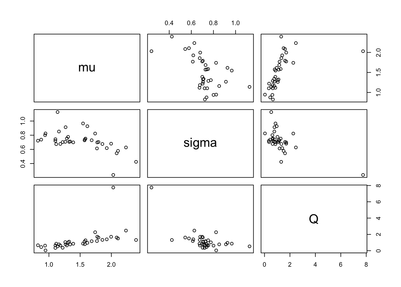
First a scatterplot:
params <- fiteach[, 4:6]
names(params) <- c("mu", "sigma", "Q")
pairs(params)
There’s one major outlier (with a high \(Q\) and low \(\sigma\)). But, even if I remove that point, the pattern looks rather more complex than just a multivariate normal. So I think that, rather than a parametric model for the kernel parameters, I’ll just draw from the “observed” values. If I wanted to get fancy I could take into account the uncertainty associated with each estimate as well… but that’s for another day (if ever).