So, last night’s analysis suggests that there’s not enough spread variability in the model. But it varied from run to run. So lets do a bunch of runs using replicate and see how far off we are.
n_init <- 50
Ler_params$gap_size <- 0
controls <- list(
  n_reps = 10,
  DS_seeds = TRUE,
  ES_seeds = TRUE,
  kernel_stoch = TRUE,
  kernel_stoch_pots = TRUE,
  seed_sampling = TRUE,
  pot_width = 7
)
The iteration and analysis, as a function to pass to replicate:
sim_mean_var <- function() {
  Adults <- matrix(n_init, controls$n_reps, 1)
  for (i in 1:6) {
    Adults <- iterate_genotype(Adults, Ler_params, controls)
  }
  npot <- ncol(Adults)
  rep_sum <- t(apply(Adults[, npot:1], 1, cummax))[, npot:1]
  maxd <- apply(rep_sum, 1, function(x) max((1:length(x))[x > 0]))
  maxd <- maxd[is.finite(maxd)]
  result <- c(mean(maxd), var(maxd))
  names(result) <- c("Mean", "Variance")
  result
}
Test the function:
sim_mean_var() Mean Variance
14.80000 13.73333 Do the replication
nruns <- 100
rep_spread_stats <- t(replicate(nruns, sim_mean_var(), simplify = TRUE))
Warning in max((1:length(x))[x > 0]): no non-missing arguments to max;
returning -Inf
Warning in max((1:length(x))[x > 0]): no non-missing arguments to max;
returning -Inf
Warning in max((1:length(x))[x > 0]): no non-missing arguments to max;
returning -Inf
Warning in max((1:length(x))[x > 0]): no non-missing arguments to max;
returning -Inf
Warning in max((1:length(x))[x > 0]): no non-missing arguments to max;
returning -Inf
Warning in max((1:length(x))[x > 0]): no non-missing arguments to max;
returning -Infrep_spread_stats Mean Variance
[1,] 14.50000 6.7222222
[2,] 13.10000 5.4333333
[3,] 15.20000 7.2888889
[4,] 18.00000 74.6666667
[5,] 14.88889 3.3611111
[6,] 16.20000 7.9555556
[7,] 13.77778 4.9444444
[8,] 13.00000 4.2222222
[9,] 14.60000 6.0444444
[10,] 19.70000 158.9000000
[11,] 16.00000 5.1111111
[12,] 13.90000 2.1000000
[13,] 14.30000 1.5666667
[14,] 14.90000 2.9888889
[15,] 15.30000 5.7888889
[16,] 16.40000 34.4888889
[17,] 15.00000 2.4444444
[18,] 15.00000 3.5555556
[19,] 15.10000 4.9888889
[20,] 14.70000 9.3444444
[21,] 15.20000 10.1777778
[22,] 14.70000 5.1222222
[23,] 17.70000 57.5666667
[24,] 16.50000 6.0555556
[25,] 14.11111 10.6111111
[26,] 13.70000 6.0111111
[27,] 13.50000 2.5000000
[28,] 17.40000 57.1555556
[29,] 13.50000 2.5000000
[30,] 14.30000 2.6777778
[31,] 14.80000 7.7333333
[32,] 14.00000 4.4444444
[33,] 15.30000 14.9000000
[34,] 17.10000 14.9888889
[35,] 14.50000 4.2777778
[36,] 15.70000 14.0111111
[37,] 13.40000 5.1555556
[38,] 15.20000 2.4000000
[39,] 14.50000 3.8333333
[40,] 13.30000 5.1222222
[41,] 14.60000 4.4888889
[42,] 19.90000 174.1000000
[43,] 15.20000 4.4000000
[44,] 13.60000 9.8222222
[45,] 15.10000 2.9888889
[46,] 14.60000 3.3777778
[47,] 14.50000 12.7222222
[48,] 16.10000 6.3222222
[49,] 17.60000 134.9333333
[50,] 15.33333 12.0000000
[51,] 13.10000 6.3222222
[52,] 14.70000 1.3444444
[53,] 15.60000 5.6000000
[54,] 15.00000 1.3333333
[55,] 17.70000 115.7888889
[56,] 15.10000 4.7666667
[57,] 13.70000 3.7888889
[58,] 15.20000 2.4000000
[59,] 14.44444 4.0277778
[60,] 14.90000 6.5444444
[61,] 15.10000 1.4333333
[62,] 15.30000 32.2333333
[63,] 14.60000 4.2666667
[64,] 14.80000 5.0666667
[65,] 13.80000 12.1777778
[66,] 15.20000 9.2888889
[67,] 15.40000 8.0444444
[68,] 14.20000 2.4000000
[69,] 14.22222 4.9444444
[70,] 15.00000 2.8888889
[71,] 21.60000 535.1555556
[72,] 15.40000 5.1555556
[73,] 15.00000 14.6666667
[74,] 14.80000 5.7333333
[75,] 14.20000 7.7333333
[76,] 14.30000 1.5666667
[77,] 14.50000 17.6111111
[78,] 14.70000 8.4555556
[79,] 13.90000 0.9888889
[80,] 16.40000 20.0444444
[81,] 14.50000 2.5000000
[82,] 15.10000 2.5444444
[83,] 15.60000 6.4888889
[84,] 17.50000 61.6111111
[85,] 14.70000 6.4555556
[86,] 14.60000 4.0444444
[87,] 14.50000 1.1666667
[88,] 14.50000 1.6111111
[89,] 16.30000 7.7888889
[90,] 14.70000 1.7888889
[91,] 15.10000 4.1000000
[92,] 15.40000 6.0444444
[93,] 14.10000 2.3222222
[94,] 14.00000 3.1111111
[95,] 14.20000 1.9555556
[96,] 15.00000 2.2222222
[97,] 14.60000 6.7111111
[98,] 14.90000 6.9888889
[99,] 14.10000 2.9888889
[100,] 15.50000 12.2777778I had to trap for cases where the population had gone extinct by gen 6.
Make a plot.
rep_spread_stats <- as.data.frame(rep_spread_stats)
maxd_data <- pull(subset(LerC_spread, Gap == "0p" & Generation == 6), Furthest)

ggplot(rep_spread_stats, aes(x = Mean)) + geom_histogram() +
  geom_vline(colour = "red", xintercept = mean(maxd_data))
`stat_bin()` using `bins = 30`. Pick better value with `binwidth`.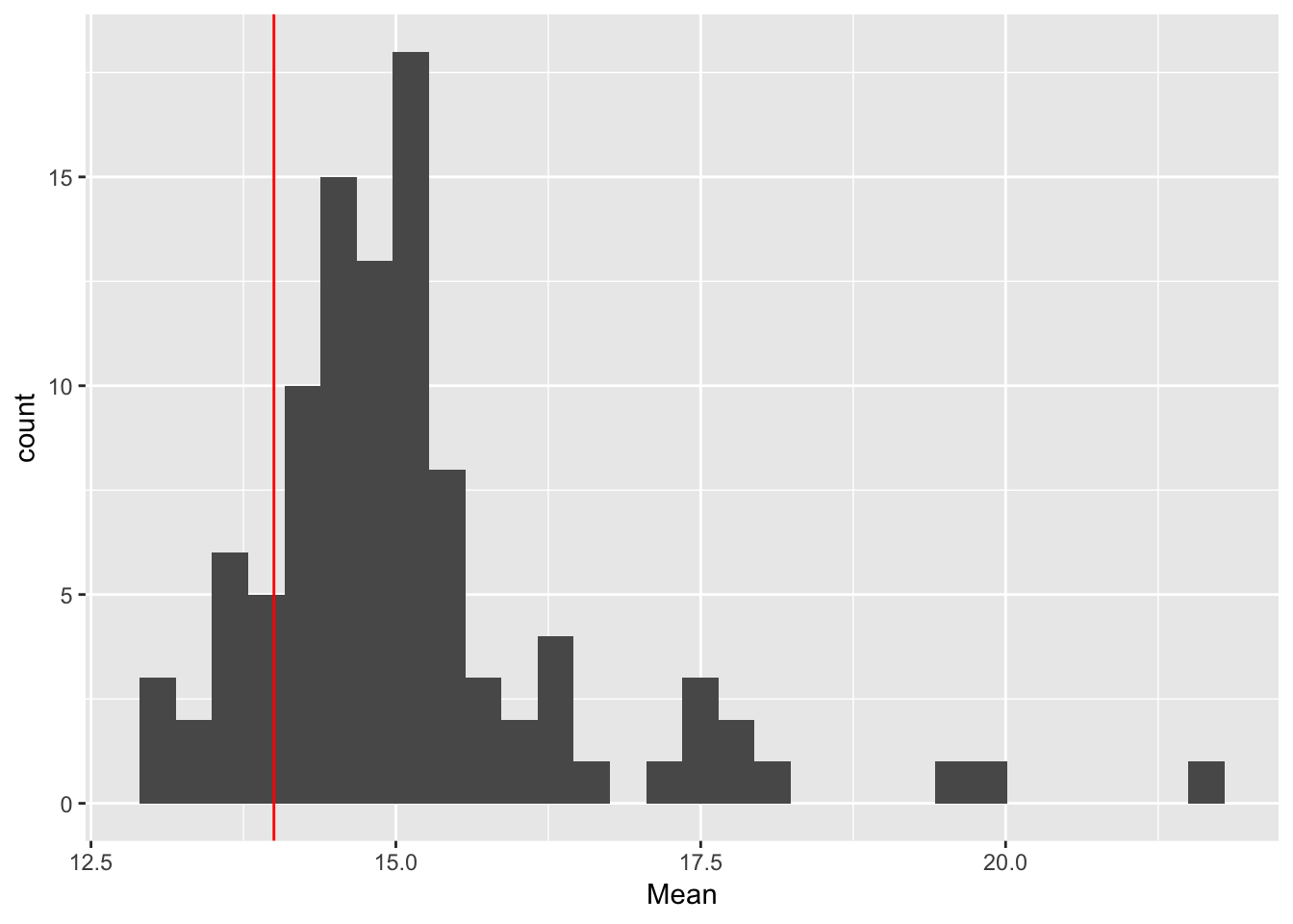
ggplot(rep_spread_stats, aes(x = Variance)) + geom_histogram() +
  geom_vline(colour = "red", xintercept = var(maxd_data))
`stat_bin()` using `bins = 30`. Pick better value with `binwidth`.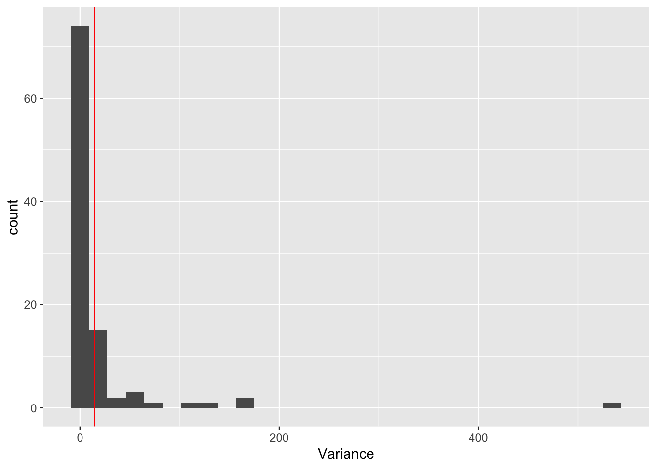 So, the distibution of variances is really skewed and there are some really large values. but the data are right in there. Here is the data: 14, 14.4444444. And here is the mean of the simulations: 15.0927778, 19.5081111. If I trim the most extreme values we get 15.0477324, 14.4353741
Just for grins, let’s see what happens if we turn off kernel stochasticity.
nruns <- 100
controls$kernel_stoch <- FALSE
rep_spread_stats <- t(replicate(nruns, sim_mean_var(), simplify = TRUE))
Warning in max((1:length(x))[x > 0]): no non-missing arguments to max;
returning -Inf
Warning in max((1:length(x))[x > 0]): no non-missing arguments to max;
returning -Inf
Warning in max((1:length(x))[x > 0]): no non-missing arguments to max;
returning -Infrep_spread_stats <- as.data.frame(rep_spread_stats)
ggplot(rep_spread_stats, aes(x = Mean)) + geom_histogram() +
geom_vline(colour = "red", xintercept = mean(maxd_data))`stat_bin()` using `bins = 30`. Pick better value with `binwidth`.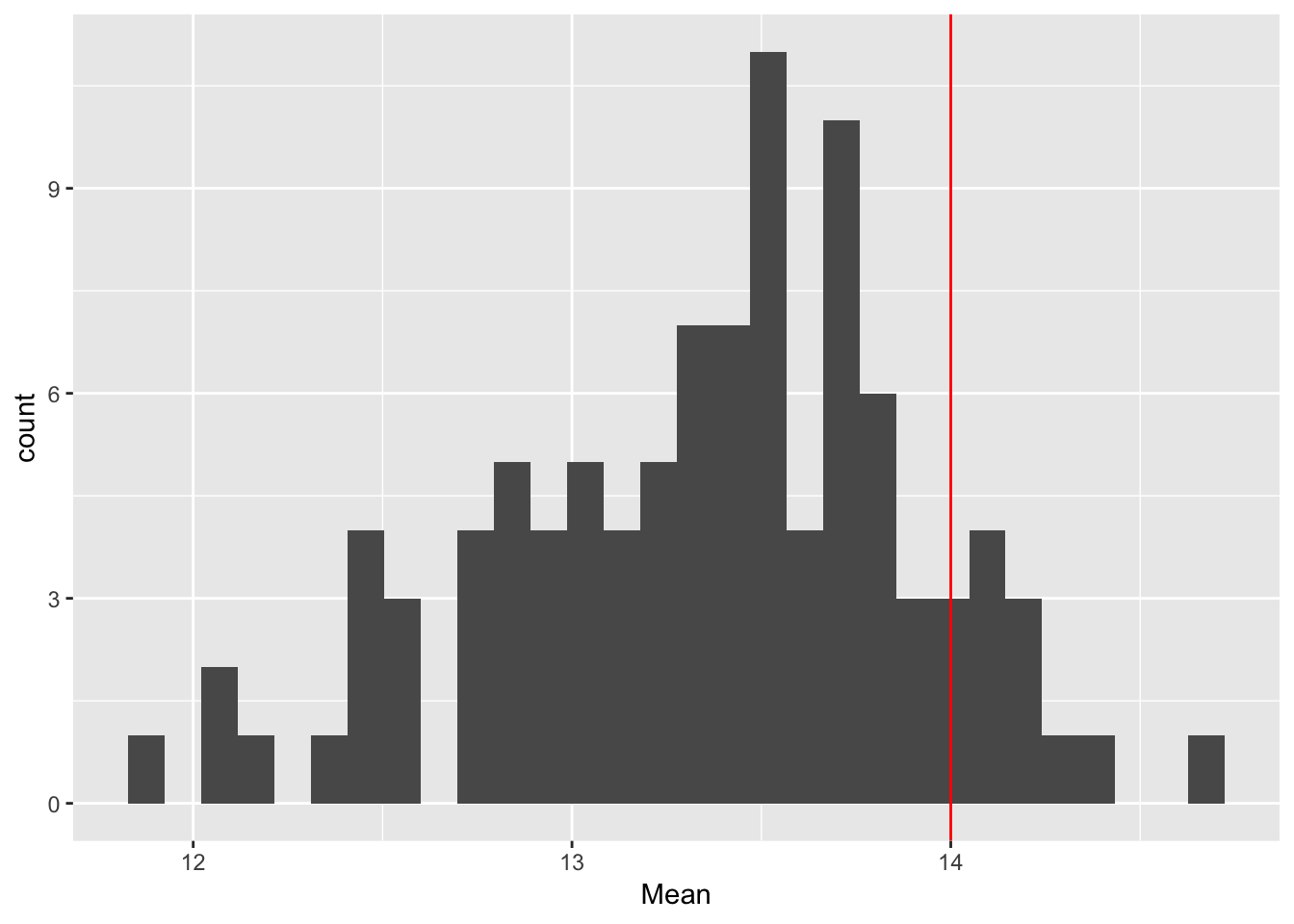
ggplot(rep_spread_stats, aes(x = Variance)) + geom_histogram() +
geom_vline(colour = "red", xintercept = var(maxd_data))`stat_bin()` using `bins = 30`. Pick better value with `binwidth`.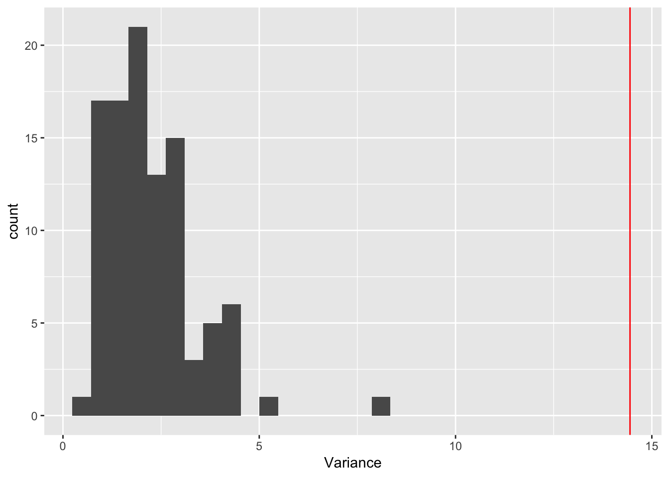 That shoots it all to heck! Let’s try shutting off the others one at a time.
No seed sampling:
nruns <- 100
controls$kernel_stoch <- TRUE
controls$seed_sampling <- FALSE
rep_spread_stats <- t(replicate(nruns, sim_mean_var(), simplify = TRUE))Warning in max((1:length(x))[x > 0]): no non-missing arguments to max;
returning -Inf
Warning in max((1:length(x))[x > 0]): no non-missing arguments to max;
returning -Inf

Warning in max((1:length(x))[x > 0]): no non-missing arguments to max;
returning -Inf

Warning in max((1:length(x))[x > 0]): no non-missing arguments to max;
returning -Inf
Warning in max((1:length(x))[x > 0]): no non-missing arguments to max;
returning -Inf
Warning in max((1:length(x))[x > 0]): no non-missing arguments to max;
returning -Infrep_spread_stats <- as.data.frame(rep_spread_stats)
ggplot(rep_spread_stats, aes(x = Mean)) + geom_histogram() +
geom_vline(colour = "red", xintercept = mean(maxd_data))`stat_bin()` using `bins = 30`. Pick better value with `binwidth`.
ggplot(rep_spread_stats, aes(x = Variance)) + geom_histogram() +
  geom_vline(colour = "red", xintercept = var(maxd_data))
`stat_bin()` using `bins = 30`. Pick better value with `binwidth`.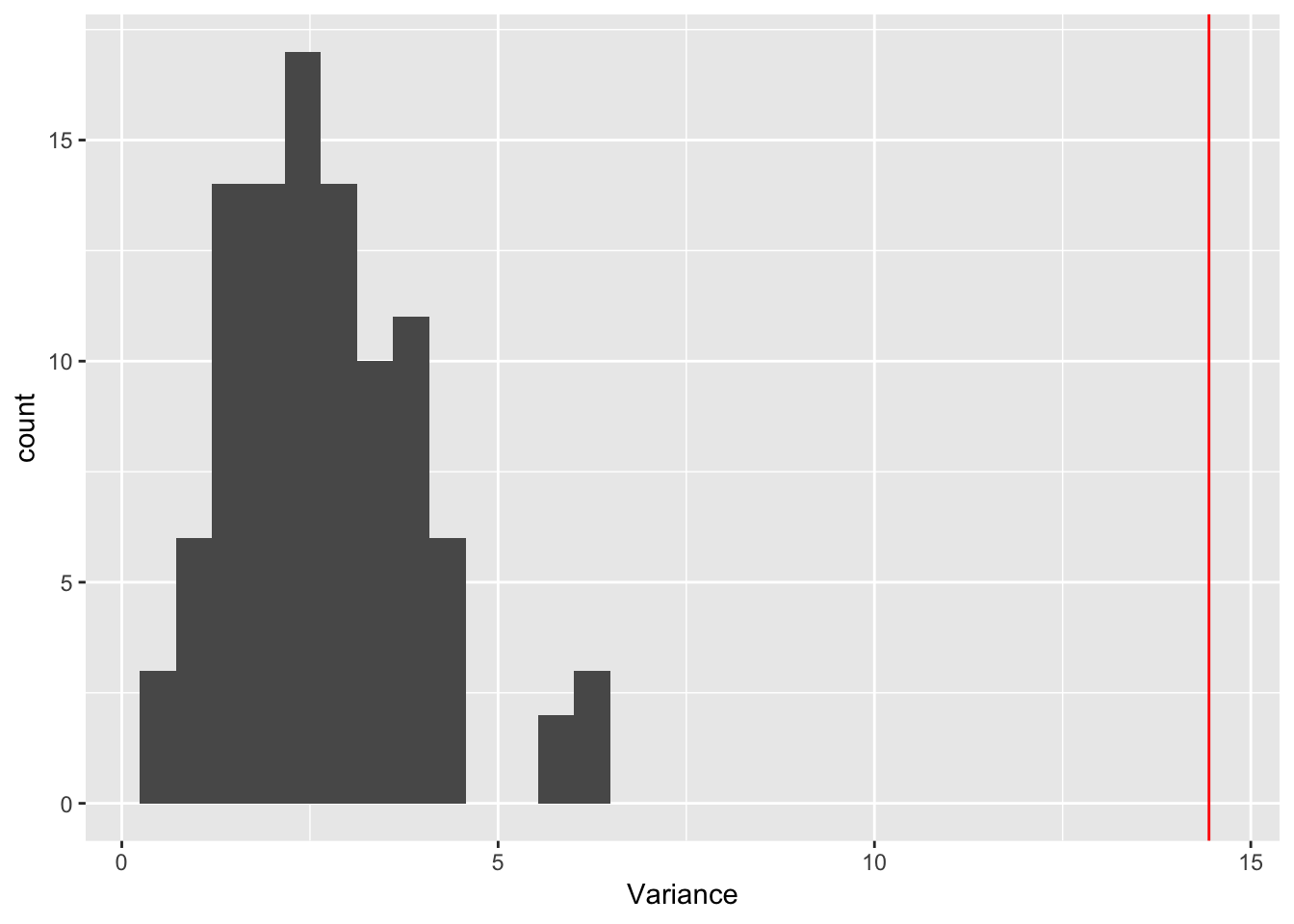
No ES:
nruns <- 100
controls$ES_seeds <- FALSE
controls$seed_sampling <- TRUE
rep_spread_stats <- t(replicate(nruns, sim_mean_var(), simplify = TRUE))rep_spread_stats <- as.data.frame(rep_spread_stats)
ggplot(rep_spread_stats, aes(x = Mean)) + geom_histogram() +
geom_vline(colour = "red", xintercept = mean(maxd_data))`stat_bin()` using `bins = 30`. Pick better value with `binwidth`.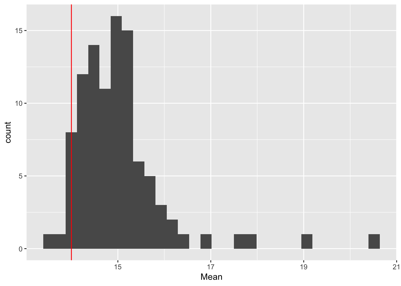
ggplot(rep_spread_stats, aes(x = Variance)) + geom_histogram() +
  geom_vline(colour = "red", xintercept = var(maxd_data))
`stat_bin()` using `bins = 30`. Pick better value with `binwidth`.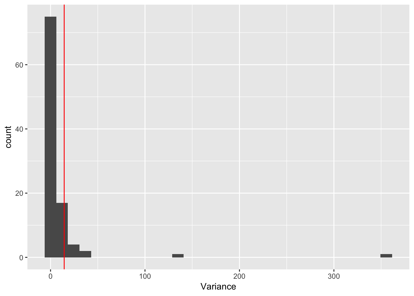
No DS:
nruns <- 100
controls$DS_seeds <- FALSE
controls$ES_seeds <- TRUE
rep_spread_stats <- t(replicate(nruns, sim_mean_var(), simplify = TRUE))rep_spread_stats <- as.data.frame(rep_spread_stats)
ggplot(rep_spread_stats, aes(x = Mean)) + geom_histogram() +
geom_vline(colour = "red", xintercept = mean(maxd_data))`stat_bin()` using `bins = 30`. Pick better value with `binwidth`.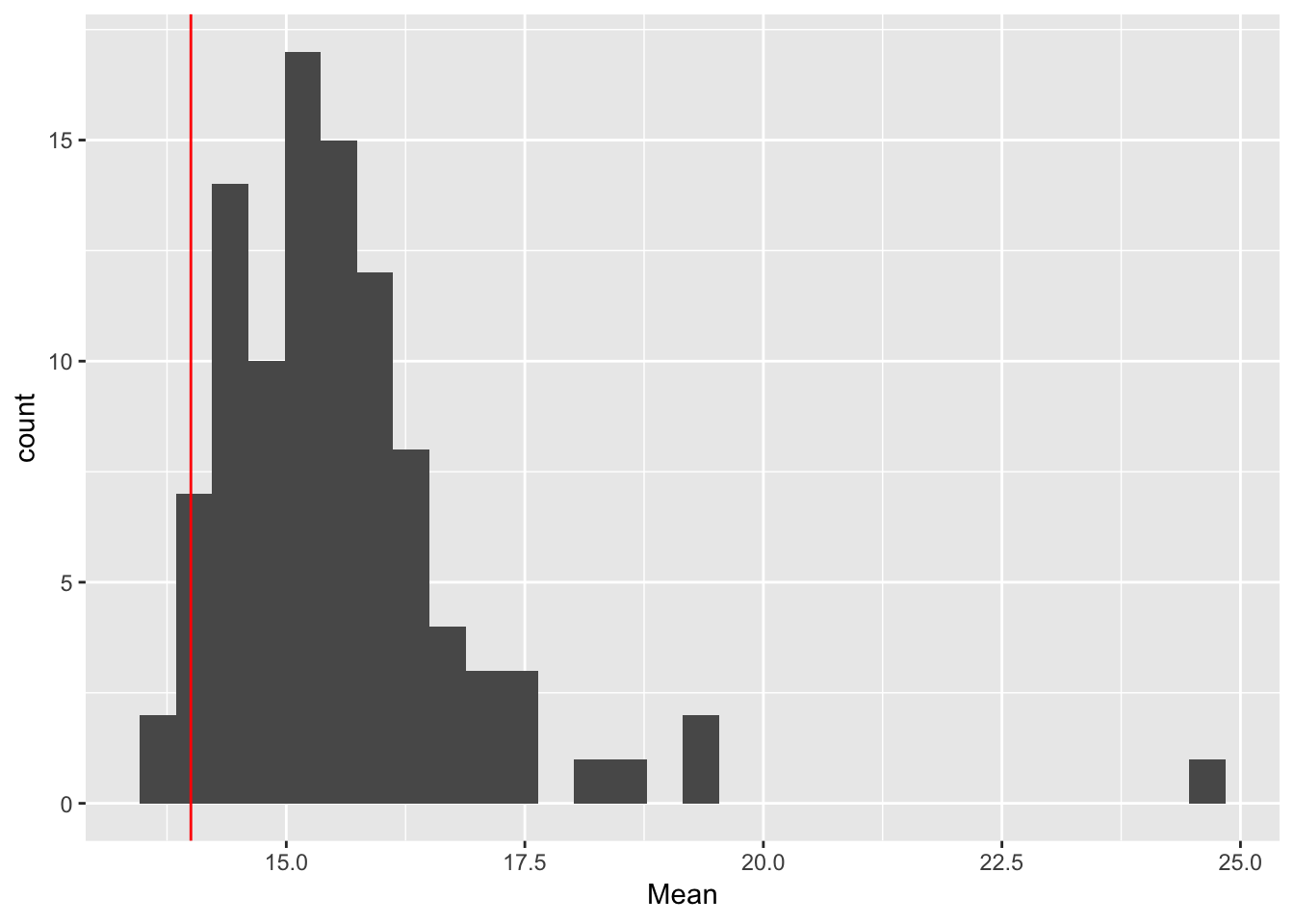
ggplot(rep_spread_stats, aes(x = Variance)) + geom_histogram() +
  geom_vline(colour = "red", xintercept = var(maxd_data))
`stat_bin()` using `bins = 30`. Pick better value with `binwidth`.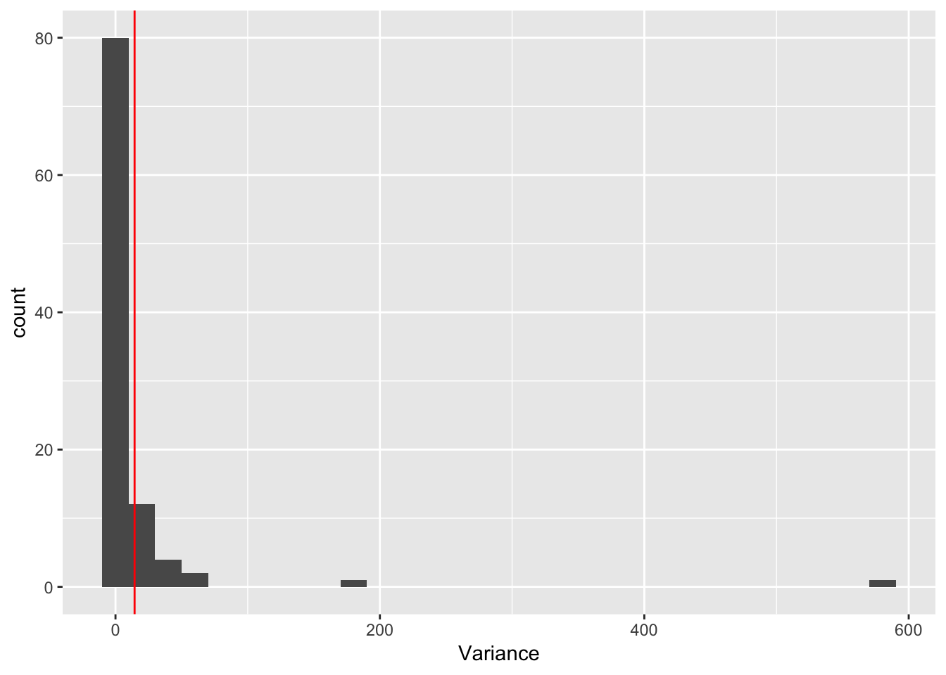
Bottom line conclusions:
- Kernel stochasticity increases the mean spread rate
- Both kernel stochasticity and seed sampling greatly increases the variance in spread rate
- Both ES and DS in seed production decrease the mean spread rate, but have little impact on the variance.